Synthetic biology with ov.synbio — from metabolism to enzyme to DNA

Synthetic biology with `ov.synbio` — from metabolism to enzyme to DNA#

This tutorial introduces omicverse.synbio, a self-contained three-layer design stack for synthetic biology: metabolic networks (A), protein / enzyme design (B), and DNA (C). Unlike a metabolism-only or a protein-only toolkit, the layers are wired together — the signature move is the A↔B hinge: predict a turnover number from an enzyme’s sequence, push it into a genome-scale metabolic model as an enzyme-capacity constraint, and re-solve the achievable yield.

Everything below runs on real data: the e_coli_core genome-scale model from BiGG, the 56-residue immunoglobulin-binding protein G B1 domain (GB1), and the real E. coli phosphofructokinase (PfkA) enzyme.

By the end you will understand:

How to load a genome-scale metabolic model (GEM), run FBA, propose strain-design targets, and read a production envelope
How the protein layer folds a sequence with ESMFold (and renders it in interactive 3D), embeds it with ESM-2, scores every point mutation with a zero-shot ESM saturation scan (visualised as a deep-mutational-scan heatmap), redesigns a backbone with ProteinMPNN, and scores thermostability ΔΔG
How to codon-optimize a gene for a host and design PCR primers
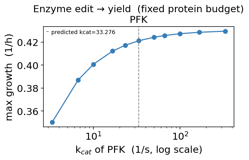
The moat — how enzyme_kcat → ec_model → fba turns an enzyme edit into a recomputed metabolic yield, plotted as a k_cat→yield curve

The protein layer uses a GPU automatically when one is available. Install with pip install 'omicverse[synbio]'.

0 — Setup#

We only import omicverse — every synbio function is accessed through ov.synbio.*, so the notebook stays terse and the API is discoverable via tab-completion on ov.synbio. Plotting helpers live in the package too (ov.synbio.plot_*, ov.synbio.view_structure), so each figure is a single call.

import omicverse as ov

ov.plot_set()
print('omicverse', ov.__version__)

🔬 Starting plot initialization...
🧬 Detecting GPU devices…
✅ NVIDIA CUDA GPUs detected: 1
    • [CUDA 0] NVIDIA H100 80GB HBM3
      Memory: 79.1 GB | Compute: 9.0

   ____            _     _    __                  
  / __ \____ ___  (_)___| |  / /__  _____________ 
 / / / / __ `__ \/ / ___/ | / / _ \/ ___/ ___/ _ \ 
/ /_/ / / / / / / / /__ | |/ /  __/ /  (__  )  __/ 
\____/_/ /_/ /_/_/\___/ |___/\___/_/  /____/\___/                                              

🔖 Version: 2.2.1rc1   📚 Tutorials: https://omicverse.readthedocs.io/
✅ plot_set complete.

omicverse 2.2.1rc1

The whole module is registered under the synthetic_biology category. ov.find_function does fuzzy search across Chinese + English aliases — this is how the omicOS agent kernel discovers synbio tools.

ov.find_function('代谢模型')   # -> ov.synbio.load_gem

🔍 Found 4 matching function(s):


1. 📦 omicverse.synbio._gem.load_gem
   📝 加载基因组尺度代谢模型 (GEM):本地 SBML 文件或 BiGG 模型 id (如 e_coli_core / iML1515) → cobra.Model。Load a genome-scale metabolic model from an SBML path or BiGG id.
   🏷️  Aliases: load_gem, 代谢模型, 基因组尺度代谢模型, 读取GEM, read_sbml, cobra_model, genome_scale_model
   📁 Category: synthetic_biology

2. 📦 omicverse.synbio._ec.ec_model
   📝 酶约束代谢模型 (GECKO / sMOMENT):把 kcat + 酶分子量转成蛋白质量预算约束。method='gecko'(默认)约束全酶促反应组(改一个酶的 kcat 会在共享蛋白预算里重新分配,物理正确);method='pool' 只约束给定反应。Enzyme-constrained model (sMOMENT/GECKO): full-proteome or targeted.
   🏷️  Aliases: ec_model, 酶约束模型, 酶约束代谢模型, enzyme_constrained_model, GECKO, ecModel, 酶约束
   📁 Category: synthetic_biology

3. 📦 omicverse.single._metabolism.Metabolism
   📝 Single-cell metabolism inference. Wraps scMetabolism (pathway activity), Compass (constraint-based reaction flux) and scFEA (graph-neural-network module flux) behind a unified method= API; results land in adata.obsm['X_metabolism'] / adata.uns['metabolism'].
   🏷️  Aliases: 代谢, metabolism, scMetabolism, 代谢活性, 代谢通量, metabolic_flux, metabolic_pathway, compass, scfea
   📁 Category: single

4. 📦 omicverse.synbio._ec.ec_model[method=gecko]
   📝 Variant of `omicverse.synbio._ec.ec_model` when `method='gecko'`.
   🏷️  Aliases: gecko, ec_model gecko, method gecko, 酶约束模型 gecko, 酶约束代谢模型 gecko, enzyme_constrained_model gecko, GECKO gecko, ecModel gecko, 酶约束 gecko
   📁 Category: synthetic_biology

<function omicverse.synbio._gem.load_gem(path_or_id: 'str', cache_dir: 'Optional[str]' = None) -> "'cobra.Model'">

1 — Layer A: genome-scale metabolic models#

load_gem accepts a local SBML file or a BiGG identifier. e_coli_core is the classic 95-reaction core-metabolism model of E. coli — small enough to be instant, real enough to be meaningful. The currency of this layer is a cobra.Model; nothing here touches AnnData.

m = ov.synbio.load_gem('e_coli_core')
print(m.id, '|', len(m.reactions), 'reactions,', len(m.genes), 'genes')

e_coli_core | 95 reactions, 137 genes

Flux Balance Analysis (FBA) maximizes the biomass reaction subject to the stoichiometric and steady-state constraints. On glucose minimal medium the model predicts a growth rate of ~0.87 h⁻¹ — the canonical answer for e_coli_core.

sol = ov.synbio.fba(m)
print('max growth =', round(sol.objective_value, 4), '/h')

max growth = 0.8739 /h

1.1 — Strain design and the production envelope#

strain_design ranks engineering targets for over-producing a metabolite. Two dependency-free engines run together: FSEOF (Flux Scanning based on Enforced Objective Flux) finds amplification targets — reactions whose flux must rise as production is enforced — and a growth-coupled knockout scan finds deletion targets. Here we target succinate (EX_succ_e).

res = ov.synbio.strain_design(m, 'EX_succ_e')
print('amplify (FSEOF):', list(res.amplify['reaction'].head(5)))
res.amplify.head()

amplify (FSEOF): ['SUCCt3', 'EX_h_e', 'FRD7', 'FUM', 'PPC']

	reaction	slope	l0	l1
0	SUCCt3	1.000000	1.638417	14.745750
1	EX_h_e	0.931367	19.092127	31.287555
2	FRD7	0.905043	0.000000	10.852285
3	FUM	0.727314	3.312901	10.852285
4	PPC	0.472126	3.897654	11.108854

Compare algorithms (side by side). method='fseof' (above) is a fast, dependency-free heuristic that ranks over-expression targets. method='optknock' runs the exact bilevel MILP OptKnock (via the StrainDesign package) — the rigorous method for concrete knockout designs.

# same target, two strain-design algorithms — side by side
fseof  = ov.synbio.strain_design(m, 'EX_succ_e', method='fseof')
oknock = ov.synbio.strain_design(m, 'EX_succ_e', method='optknock', max_knockouts=2, time_limit=90)
print("COMPARISON — succinate over-production design")
print("  method='fseof'    (heuristic) amplify targets:", list(fseof.amplify['reaction'].head(3)))
print("  method='optknock' (exact StrainDesign MILP) knockout designs:")
print(oknock.knockout.head(3).to_string(index=False))

COMPARISON — succinate over-production design
  method='fseof'    (heuristic) amplify targets: ['SUCCt3', 'EX_h_e', 'FRD7']
  method='optknock' (exact StrainDesign MILP) knockout designs:
knockouts  n_knockouts
 [ICDHyr]            1
   [GLNS]            1
  [PIt2r]            1

The top amplification targets — FRD7 (fumarate reductase), FUM (fumarase), PPC (PEP carboxylase) — are exactly the enzymes a metabolic engineer would over-express to push carbon toward succinate.

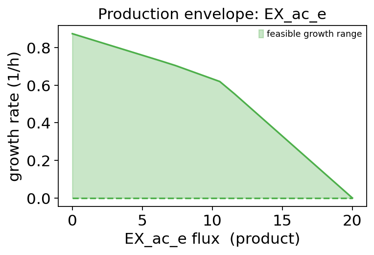
The production envelope makes the growth–production trade-off explicit: for acetate (EX_ac_e), the feasible growth rate shrinks as we force more product secretion — the fundamental tension every strain design must navigate.

ov.synbio.plot_production_envelope(m, 'EX_ac_e')
None

../_images/a03dc90ca526405e19f881fbf250156f67c8930fc610f2e7b95637d65a1d264d.png

2 — Layer B: protein & enzyme design (GPU)#

The protein layer is built on public state-of-the-art open models — ESM-2 / ESM-1v / ESMFold and ProteinMPNN. Each function prints the device it actually used, so you can confirm the GPU is engaged. Our test protein is the 56-residue GB1 domain — a small, well-folded natural protein.

GB1 = 'MTYKLILNGKTLKGETTTEAVDAATAEKVFKQYANDNGVDGEWTYDDATKTFTVTE'
len(GB1)

2.1 — ESM-2 embeddings#

protein_embed returns a fixed-length vector per sequence (mean-pooled residue representations from ESM-2). These feed any downstream model — property regressors, clustering, function transfer.

X = ov.synbio.protein_embed([GB1], model='esm2_t33_650M')
X.shape          # (1, 1280)

[ov.synbio.protein_embed] model=esm2_t33_650M device=cuda (NVIDIA H100 80GB HBM3, 79 GB)

(1, 1280)

2.2 — Zero-shot variant effect (in-silico directed evolution)#

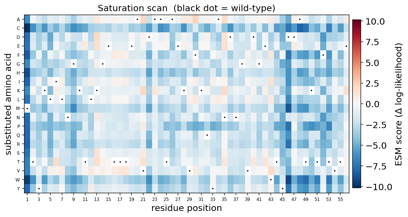
variant_effect scores substitutions with an ESM language model — no labels needed. With mutations=None it runs a full saturation scan (every position × 19 alternatives): a computational deep-mutational-scan. A positive score means the model prefers the mutant.

dms = ov.synbio.variant_effect(GB1, model='esm1v')
print('scored', len(dms), 'substitutions')
dms.head()          # most-favoured substitutions first

[ov.synbio.variant_effect] model=esm1v scoring=masked-marginals device=cuda (NVIDIA H100 80GB HBM3, 79 GB)
scored 1064 substitutions

	mutation	wt	pos	mut	score
0	F30A	F	30	A	2.283173
1	V21A	V	21	A	2.167181
2	V21K	V	21	K	2.088095
3	W43V	W	43	V	2.042460
4	K13D	K	13	D	2.005156

plot_variant_effect renders the whole scan as a deep-mutational-scan heatmap (position × amino acid). Blue columns are conserved (few tolerated substitutions); red cells are substitutions the model favours. Black dots mark the wild-type residue at each position.

ov.synbio.plot_variant_effect(dms)
None

../_images/6b250b4d64df4ed95253e5d85234d6d19327accc593ca9f5f1613ddc6a1b98d7.png

2.3 — Structure prediction with ESMFold#

predict_structure folds a single sequence into 3D coordinates with ESMFold (no MSA). It requires a GPU by default. The mean pLDDT (0–100) reports model confidence — GB1 is a well-behaved domain and scores high.

pred = ov.synbio.predict_structure(GB1, out_path='gb1.pdb')
print('mean pLDDT =', round(pred.mean_plddt, 1), '| device =', pred.device)

[ov.synbio.predict_structure] device=cuda (NVIDIA H100 80GB HBM3, 79 GB) len=56
[ov.synbio.predict_structure] done: mean pLDDT=89.0
mean pLDDT = 89.0 | device = cuda

view_structure renders it as an interactive 3D cartoon (py3Dmol), coloured by pLDDT confidence bands (blue = very high, orange = low). Drag to rotate; the view persists in the exported HTML docs.

ov.synbio.view_structure(pred)

3Dmol.js failed to load for some reason. Please check your browser console for error messages.

<py3Dmol.view at 0x7f1110eb3ca0>

2.4 — Inverse design (ProteinMPNN) and thermostability ΔΔG#

Given the backbone we just folded, inverse_design (ProteinMPNN) samples new sequences predicted to adopt the same fold — the inverse problem of folding. A lower ProteinMPNN score is more confident; good designs beat the native sequence’s score.

designs = ov.synbio.inverse_design('gb1.pdb', num_sequences=4)
print('native score:', round(designs[0].score, 3),
      '| best design score:', round(designs[1].score, 3))

[ov.synbio.inverse_design] method=proteinmpnn backbone=gb1.pdb device=cuda (NVIDIA H100 80GB HBM3, 79 GB) n=4
native score: 1.344 | best design score: 0.859

stability_ddg estimates how a point mutation changes fold stability, using the ProteinMPNN log-likelihood ΔΔG proxy (a positive value = predicted destabilizing).

ddg = ov.synbio.stability_ddg('gb1.pdb', mutations=['T2V', 'K4E', 'L5A'])
ddg

[ov.synbio.stability_ddg] pdb=gb1.pdb method=proteinmpnn device=cuda (NVIDIA H100 80GB HBM3, 79 GB)

	mutation	wt	pos	mut	ddg_proxy
0	L5A	L	5	A	5.038882
1	K4E	K	4	E	1.367056
2	T2V	T	2	V	1.047549

Compare algorithms. The default method='proteinmpnn' is a zero-shot log-likelihood ΔΔG proxy (no training labels). method='thermompnn' runs the real ThermoMPNN model (Dieckhaus 2024) — a stability head trained on the mega-scale dataset — giving calibrated ΔΔG in kcal/mol (positive = destabilising). ThermoMPNN is auto-cloned on first use.

cmp = ov.synbio.stability_ddg('gb1.pdb', mutations=['T2V','K4E','L5A'], method='thermompnn')
print('ThermoMPNN (real, trained) ΔΔG kcal/mol:')
cmp

[ov.synbio.stability_ddg] pdb=gb1.pdb method=thermompnn device=cuda (NVIDIA H100 80GB HBM3, 79 GB)
ThermoMPNN (real, trained) ΔΔG kcal/mol:

	mutation	wt	pos	mut	ddg
0	L5A	L	5	A	2.379662
1	K4E	K	4	E	1.627585
2	T2V	T	2	V	-0.224619

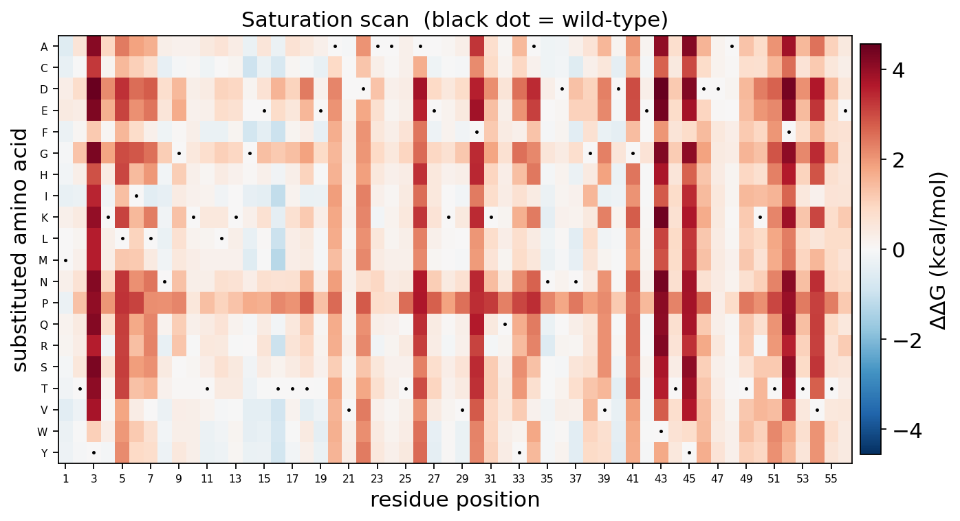
Run the full ThermoMPNN saturation scan and view it as a ΔΔG heatmap — the same plot_variant_effect helper, now on calibrated kcal/mol values. Red = destabilising, blue = stabilising; buried positions light up as intolerant columns.

ssm = ov.synbio.stability_ddg('gb1.pdb', method='thermompnn')   # full saturation scan
ov.synbio.plot_variant_effect(ssm)                              # real ΔΔG landscape (kcal/mol)
None

[ov.synbio.stability_ddg] pdb=gb1.pdb method=thermompnn device=cuda (NVIDIA H100 80GB HBM3, 79 GB)

../_images/80d7f38f2eb37de361fb51fa98e4ec891e0a0eb1db91aae50b7aec548096b66a.png

3 — Layer C: DNA design#

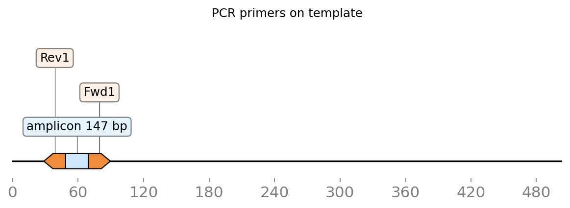
To actually build a protein you need a gene. codon_optimize rewrites a sequence for a host’s codon usage while respecting GC bounds and removing unwanted restriction sites (DNAchisel). design_primers then designs validated PCR primer pairs (primer3).

opt = ov.synbio.codon_optimize(GB1, host='e_coli')
print(opt)
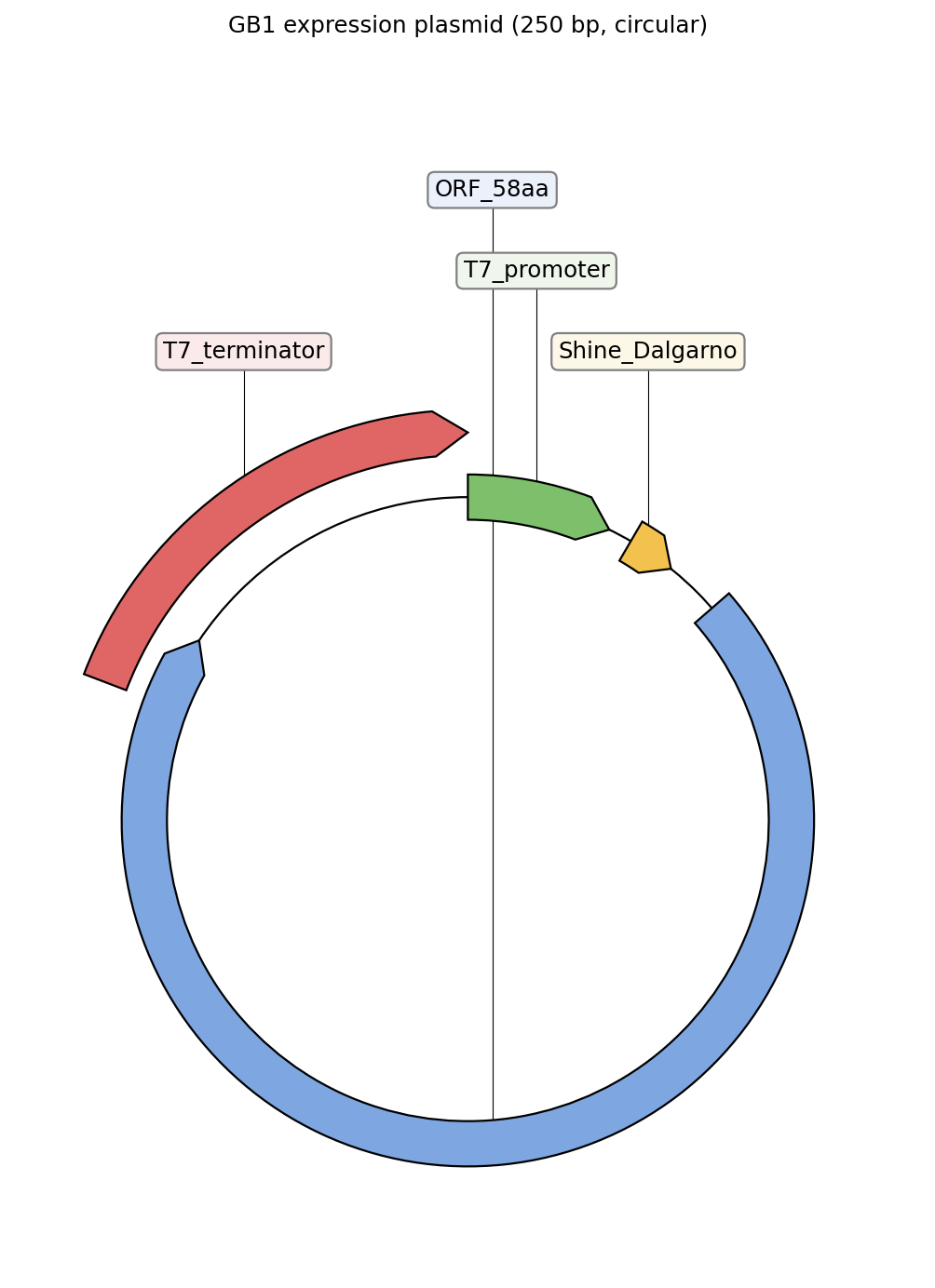
# wrap the codon-optimised gene in a T7 expression cassette and view it as a plasmid map
cassette = ('TAATACGACTCACTATAGG' + 'AAAGGAGGACAACAT' + opt.sequence
            + 'CTAGCATAACCCCTTGGGGCCTCTAAACGGGTCTTGAGGGGTTTTTTG')
ov.synbio.view_construct(cassette, circular=True, title='GB1 expression plasmid')
None

CodonResult(host='e_coli', len=168, edits=36, GC=0.51, constraints_ok=True)

../_images/7e167555fc5060ad600ff2f77c8fb971229983dd47777467c7c1ceed70d99d7f.png

# design PCR primers and draw them as binding arrows on the template (amplicon highlighted)
primers = ov.synbio.design_primers(opt.sequence * 3)   # tripled so a product fits
print('cloning primers:', primers[0])
ov.synbio.view_primers(opt.sequence * 3, primers[0])
None

cloning primers: PrimerPair(product=147bp, Tm=60.0/60.1, L=CGACCGCGGAAAAAGTGTTT, R=TGGTTTCGCCTTTCAGGGTT)

../_images/048c37585e8446397f6ed299c613476ca189b4829d1e2fe61bcc8ecd5a17719a.png

4 — The moat: A↔B coupling#

Here is the feature a metabolism-only or protein-only tool can’t offer: edit an enzyme, and the metabolic network re-solves its yield.

We start from the real E. coli phosphofructokinase (PfkA) sequence and its physiological substrate fructose-6-phosphate. enzyme_kcat predicts a turnover number k_cat; ec_model turns {reaction: k_cat} into an enzyme-capacity constraint (a lightweight GECKO); fba re-solves growth under that constraint.

PFKA = ('MIKKIGVLTSGGDAPGMNAAIRGVVRSALTEGLEVMGIYDGYLGLYEDRMVQLDRYSVSDMINRGGTFLGSARFPEFRD'
        'ENIRAVAIENLKKRGIDALVVIGGDGSYMGAMRLTEMGFPCIGLPGTIDNDIKGTDYTIGFFTALSTVVEAIDRLRDT')
F6P = 'OCC1OC(O)(COP(=O)(O)O)C(O)C1O'
k = ov.synbio.enzyme_kcat(PFKA, F6P)
print('predicted kcat(PfkA) =', round(k.kcat, 2), '/s')

[ov.synbio.enzyme_kcat] method=baseline device=cuda (NVIDIA H100 80GB HBM3, 79 GB)
predicted kcat(PfkA) = 33.28 /s

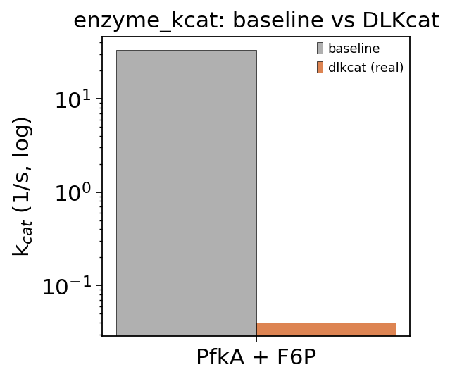
Compare algorithms. The k_cat above is the sequence-sensitive baseline. method='dlkcat' runs the real trained DLKcat model (Li 2022) — a substrate-graph GNN fused with a protein-sequence CNN — for a calibrated turnover number (needs the substrate SMILES).

# k_cat: sequence baseline vs the REAL trained DLKcat model — side by side
kb = ov.synbio.enzyme_kcat(PFKA, F6P, method='baseline', verbose=False)
kd = ov.synbio.enzyme_kcat(PFKA, F6P, method='dlkcat', verbose=False)   # substrate-graph GNN + protein CNN
print(f"baseline (ESM heuristic) = {kb.kcat:.2f} /s   |   dlkcat (real trained) = {kd.kcat:.3f} /s")
ov.synbio.plot_method_comparison(['PfkA + F6P'],
    {'baseline': [kb.kcat], 'dlkcat (real)': [kd.kcat]},
    ylabel='k$_{cat}$ (1/s, log)', title='enzyme_kcat: baseline vs DLKcat', log=True)
None

baseline (ESM heuristic) = 33.28 /s   |   dlkcat (real trained) = 0.040 /s

../_images/3ce788722e06c850dd20eca15e16b8907d17f48676cff62135582503ed8f81f2.png

ecm = ov.synbio.ec_model(m, {'PFK': k.kcat})
print('growth under enzyme constraint =', round(ov.synbio.fba(ecm).objective_value, 4), '/h')

growth under enzyme constraint = 0.4212 /h

Compare formulations (side by side). ec_model defaults to method='gecko' — the real full-proteome sMOMENT/GECKO, where all 69 enzymatic reactions compete for a shared protein-mass budget (so it lowers max growth, exactly as published ecModels do). method='pool' constrains only the listed reaction — lighter, but blind to proteome competition.

# same PFK kcat, two enzyme-constraint formulations — side by side
g_free  = ov.synbio.fba(m).objective_value
g_gecko = ov.synbio.fba(ov.synbio.ec_model(m, {'PFK': k.kcat}, method='gecko')).objective_value
g_pool  = ov.synbio.fba(ov.synbio.ec_model(m, {'PFK': k.kcat}, method='pool')).objective_value
print('COMPARISON — max growth /h under each formulation')
print(f"  unconstrained FBA                         : {g_free:.3f}")
print(f"  ec_model method='gecko' (full proteome)   : {g_gecko:.3f}   <- default, real sMOMENT/GECKO")
print(f"  ec_model method='pool'  (only PFK)        : {g_pool:.3f}")

COMPARISON — max growth /h under each formulation
  unconstrained FBA                         : 0.874
  ec_model method='gecko' (full proteome)   : 0.421   <- default, real sMOMENT/GECKO
  ec_model method='pool'  (only PFK)        : 0.848

Now sweep the enzyme’s k_cat under the same protein budget — imagine slower or engineered-faster variants. plot_enzyme_yield_response builds an enzyme-constrained model at each k_cat and re-solves growth. A faster enzyme needs less protein per unit flux, so the capacity constraint relaxes and attainable growth rises until it plateaus at the unconstrained optimum. That is a quantitative link from sequence → phenotype — the ov.synbio moat, in one figure.

fig, curve = ov.synbio.plot_enzyme_yield_response(m, 'PFK', base_kcat=k.kcat)
curve.head()

	kcat	growth
0	3.328	0.350191
1	6.655	0.387082
2	9.983	0.400752
3	16.638	0.412246
4	23.293	0.417334

../_images/48e145600ce9eac1dc3538d8321d80cd7f23054953bce0f60a675c250feacb0a.png

Summary#

In one notebook we went from a metabolic network (FBA, strain design, production envelope) through protein/enzyme design (embeddings, saturation-scan heatmap, ESMFold structure in interactive 3D, ProteinMPNN redesign, ΔΔG) to DNA (codon optimization, primers) — and closed the loop with the A↔B hinge, where an enzyme’s predicted k_cat reshapes the metabolic yield.

Baseline → SOTA via method=. Following the omicverse convention, every task is one function; swapping in a state-of-the-art backend is just a method= value (never a new function):

stability_ddg(..., method='thermompnn') — real trained ThermoMPNN (calibrated ΔΔG), vs the default ProteinMPNN proxy (shown above).
enzyme_function(seq, method='clean') — real CLEAN EC-number model, vs the knn baseline.
strain_design(m, target, method='optknock') — exact StrainDesign MILP, vs the fseof heuristic.
ec_model(m, kcat, method='gecko') — full-proteome GECKO (the default), vs method='pool'.
rbs_strength(utr, method='ostir') — the OSTIR RBS Calculator; reaction_dg(rxn, method='equilibrator') for eQuilibrator.

Where to go next:

Swap e_coli_core for a genome-scale model such as iML1515, or your own SBML.
Feed variant_effect / stability_ddg rankings back into enzyme_kcat → ec_model to screen enzyme variants in silico for pathway yield.

Every function is registered under synthetic_biology — run ov.list_functions(category='synthetic_biology') to see the full surface.