
Molecular dynamics — from a static model to motion#
ov.mol hands you a structure (fetch_structure), a pocket
(pockets) and a docked pose (dock). Every one of those is a
snapshot, and a snapshot cannot answer the questions that decide whether a
result is real:
is this AlphaFold fold actually stable, and which parts are floppy?
does that docked pose survive more than a picosecond of thermal motion?
what is the binding energy averaged over an ensemble, rather than read off one rigid-receptor pose?
Molecular dynamics supplies the missing time axis. This notebook runs the arc end to end on real targets — ubiquitin (1UBQ) and EGFR (1M17).
Hardware. MD is GPU work. Every call prints the OpenMM platform it resolved; if it says
CPUwhere you expectedCUDA, see the install notes in the module index. Timings below are from an NVIDIA H100.
0. Setup#
The dynamics layer needs the [md] extra (OpenMM + MDTraj). PDBFixer, which
repairs structures before simulation, is vendored inside omicverse and never
needs installing.
pip install 'omicverse[md]'
# on a GPU box prefer the conda-forge CUDA build:
conda install -c conda-forge openmm mdtraj
import omicverse as ov
import matplotlib.pyplot as plt

ov.plot_set()
🔬 Starting plot initialization...
🧬 Detecting GPU devices…
🚫 PyTorch not available - GPU detection skipped

   ____            _     _    __
  / __ \____ ___  (_)___| |  / /__  _____________
 / / / / __ `__ \/ / ___/ | / / _ \/ ___/ ___/ _ \
/ /_/ / / / / / / / /__ | |/ /  __/ /  (__  )  __/
\____/_/ /_/ /_/_/\___/ |___/\___/_/  /____/\___/

🔖 Version: 2.2.4rc1   📚 Tutorials: https://omicverse.readthedocs.io/
✅ plot_set complete.
1. The target#
Ubiquitin — 76 residues, the standard MD benchmark, and small enough that a nanosecond costs a couple of minutes.
s = ov.mol.fetch_structure('1UBQ', source='pdb')
s
MolStructure(1UBQ, source=pdb, 76 residues)
2. Run it — one call#
ov.mol.simulate chains everything a correct run needs: repair the structure
and add hydrogens at pH 7, parameterise with Amber14, solvate in a TIP3P box
with 0.15 M NaCl, minimise, equilibrate (NVT then NPT with a released
restraint), and produce the trajectory.
Watch the printed platform line and the Speed (ns/day) column.
traj = ov.mol.simulate(s, ns=1.0, outdir='md_ubiquitin', seed=0)
traj
🧬 ov.mol.simulate — 1 ns, output in md_ubiquitin/
fixing structure (receptor_input.pdb) at pH 7.0
solvating: tip3p box, padding 1.0 nm, 0.15 M Na+/Cl-
system ready: 17081 particles (explicit solvent)
   OpenMM platform: CUDA (precision=mixed)
minimisation: -99592.7 -> -285852.1 kJ/mol
OpenMM platform: CUDA (precision=mixed)
NVT 100 ps @ 300 K (restraint 'heavy', k=1000)
NPT 100 ps @ 1 bar (restraint released linearly)
equilibrated: potential energy -232677.6 kJ/mol
OpenMM platform: CUDA (precision=mixed)
production: 1 ns, 500000 steps @ 2 fs, NPT, frame every 10 ps -> md_ubiquitin/prod.dcd
#"Step"	"Time (ps)"	"Potential Energy (kJ/mole)"	"Temperature (K)"	"Box Volume (nm^3)"	"Density (g/mL)"	"Speed (ns/day)"	"Time Remaining"
50000	99.99999999994834	-233564.2536023378	299.01065209373735	171.4054476698042	1.0113650064688766	0	--
100000	200.00000000022686	-232923.72501580347	301.4364302582894	170.71471229873293	1.015457129365756	74.8	15:23
150000	300.00000000070435	-233340.30847860873	300.6692408255923	170.8373831629241	1.014727973947298	76.1	13:14
200000	400.00000000118183	-233597.09100499412	299.7872161138524	169.9191030670751	1.0202117864460563	72.5	11:54
250000	500.0000000016593	-232933.93393933366	299.20827049376857	171.3459351158509	1.0117162777988518	68.7	10:29
300000	599.9999999996356	-232655.47322768508	302.7226911554526	171.66724610651085	1.0098226401547512	73.8	7:48
350000	699.999999997271	-233300.3243274265	299.49027277836115	170.842488809787	1.0146976486884414	77.5	5:34
400000	799.9999999949063	-232937.44707820425	299.96662720848497	170.21140490262513	1.0184597899920078	78.5	3:40
450000	899.9999999925416	-232695.65316536056	299.75541546805823	169.84924766711427	1.0206313779565621	79	1:49
500000	999.9999999901769	-233852.20380115113	299.3339179114926	171.1157256442279	1.0130773839676017	79.5	0:00
done: 100 frames on platform CUDA
MDTrajectory(100 frames, 1.000 ns @ 10 ps/frame, 'prod.dcd')
p = traj.provenance
p['platform'], p['precision'], p['forcefield'], p['water'], p['ensemble']
('CUDA', 'mixed', 'amber14-all', 'tip3p', 'NPT')
3. Did it stay folded?#
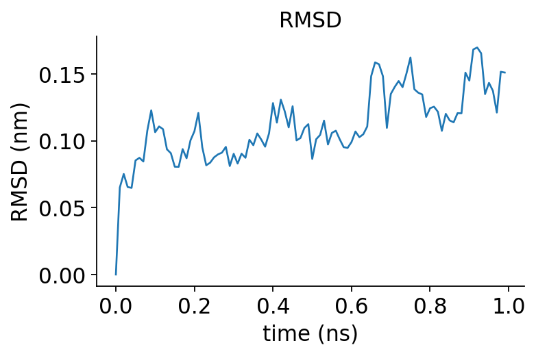
RMSD against the starting frame is the first thing to read. A stable domain rises quickly and then plateaus — typically 0.1–0.3 nm. A curve that keeps climbing means the structure is coming apart.
ax = ov.mol.plot_rmsd(traj)
plt.show()
r = ov.mol.rmsd(traj)
print(f'CA-RMSD  mean {r.mean():.3f} nm | final {r[-1]:.3f} | max {r.max():.3f}')
CA-RMSD mean 0.111 nm | final 0.151 | max 0.170
4. Where is it flexible?#
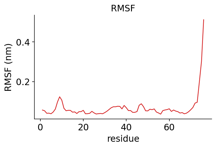
RMSF is the per-residue flexibility profile — the physics-based answer to “which parts of my model are floppy?”, complementary to pLDDT (which is only the predictor’s own confidence).
ax = ov.mol.plot_rmsf(traj)
plt.show()
import numpy as np
f = ov.mol.rmsf(traj)
print('most flexible residues:', (np.argsort(f)[-5:] + 1).tolist())
print(f'core RMSF {np.median(f):.3f} nm vs peak {f.max():.3f} nm')
most flexible residues: [10, 9, 74, 75, 76]
core RMSF 0.053 nm vs peak 0.512 nm
The peak should land on the C-terminal Leu73-Arg74-Gly75-Gly76 tail — the segment ubiquitin uses to conjugate onto substrates, and which is genuinely disordered in solution. That the simulation finds it without being told is a good sign the setup is sound.
5. Compactness and secondary structure#
Radius of gyration tracks global size; DSSP tracks whether the helices and sheets survive.
ax = ov.mol.plot_rg(traj)
plt.show()

rg = ov.mol.radius_of_gyration(traj)
ss = ov.mol.secondary_structure(traj)
print(f'Rg {rg.mean():.3f} +/- {rg.std():.3f} nm   (ubiquitin, literature ~1.17)')
print(f'helix {(ss == "H").mean():.2f} | sheet {(ss == "E").mean():.2f} | coil {(ss == "C").mean():.2f}')
Rg 1.185 +/- 0.008 nm   (ubiquitin, literature ~1.17)
helix 0.19 | sheet 0.34 | coil 0.47
6. Which contacts actually persist?#
Hydrogen bonds present in most frames — the interactions holding the fold together (or, for a complex, holding the ligand in place).
hb = ov.mol.hbonds(traj, freq=0.6)
print(f'{len(hb)} hydrogen bonds present in >60% of frames')
hb.head()
50 hydrogen bonds present in >60% of frames
| donor_residue | donor_atom | hydrogen | acceptor_residue | acceptor_atom | occupancy | |
|---|---|---|---|---|---|---|
| 0 | PHE4 | N | H | SER65 | O | 1.0 |
| 1 | VAL5 | N | H | ILE13 | O | 1.0 |
| 2 | ILE23 | N | H | ARG54 | O | 1.0 |
| 3 | VAL17 | N | H | MET1 | O | 1.0 |
| 4 | ASP21 | N | H | GLU18 | O | 1.0 |
7. Conformational states#
Clustering the frames by pairwise RMSD finds the distinct states visited. The
medoid frames are representative structures you can send back to
ov.mol.view.
labels, medoids = ov.mol.cluster(traj, n_clusters=3)
print('cluster sizes:', [int((labels == c).sum()) for c in sorted(set(labels))])
print('representative frames:', medoids.tolist())
cluster sizes: [26, 36, 38]
representative frames: [51, 88, 15]
8. Stage-by-stage control — when the defaults are not what you want#
simulate is an orchestration of four functions. Call them yourself for a
different restraint scheme, a longer equilibration, implicit solvent, or a
4 fs timestep with hydrogen-mass repartitioning.
Implicit solvent (GBn2) drops the water box entirely — far faster, and a good choice for long sampling when explicit solvation structure does not matter.
sysobj = ov.mol.prepare_system(s, water='implicit', hmr=True, seed=0)
sysobj
MDSystem(1231 atoms, amber14-all/implicit)
Minimisation is not optional — it relieves the clashes left by
structure repair and solvation. Skipping it is the most common cause of a
Particle coordinate is NaN blow-up.
sysobj = ov.mol.minimize(sysobj)
OpenMM platform: CUDA (precision=mixed)
minimisation: -1865.4 -> -14500.6 kJ/mol
sysobj = ov.mol.equilibrate(sysobj, nvt_ps=100, npt_ps=0, seed=0)
OpenMM platform: CUDA (precision=mixed)
NVT 100 ps @ 300 K (restraint 'heavy', k=1000)
equilibrated: potential energy -10773.0 kJ/mol
hmr=True allows a 4 fs timestep instead of 2 fs, roughly
doubling throughput. The guard refuses 4 fs on a system built without HMR,
because it would be unstable.
traj2 = ov.mol.production(sysobj, ns=2.0, timestep_fs=4.0, ensemble='NVT',
                          report_ps=10.0, traj='md_implicit/prod.dcd', seed=0)
traj2
OpenMM platform: CUDA (precision=mixed)
   production: 2 ns, 500000 steps @ 4 fs, NVT, frame every 10 ps -> md_implicit/prod.dcd
#"Step"	"Time (ps)"	"Potential Energy (kJ/mole)"	"Temperature (K)"	"Speed (ns/day)"	"Time Remaining"
50000	199.9999999998967	-10837.636051786785	302.32555650739266	0	--
100000	400.0000000004537	-10599.096309643399	292.64286698955556	88.5	26:02
150000	600.0000000014087	-10714.410527386057	308.2034512645991	83.2	24:13
200000	800.0000000023637	-10742.994739162843	293.88880583159647	78.4	22:03
250000	1000.0000000033186	-10601.246048079225	301.013883585517	77	18:42
300000	1199.9999999992713	-10587.21834106349	305.8388718996018	76.5	15:03
350000	1399.999999994542	-10676.13455149457	296.04416867530966	76.3	11:19
400000	1599.9999999898125	-10865.177639652553	311.4517413583805	77.6	7:25
450000	1799.9999999850832	-10651.282804505581	304.115226527518	75.7	3:48
500000	1999.9999999803538	-10714.889314835986	305.3955572334219	74.5	0:00
done: 200 frames on platform CUDA
MDTrajectory(200 frames, 2.000 ns @ 10 ps/frame, 'prod.dcd')
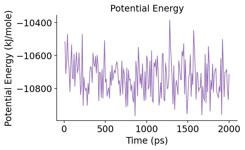
ax = ov.mol.plot_energy(traj2)
plt.show()
9. dock → MD → MM-GBSA — rescoring a pose with dynamics#
This is the part docking alone cannot do.
ov.mol.dock returns a static pose with a Vina score: a single-point
estimate on a rigid receptor. What we want to know is whether the pose
stays, and what the binding energy looks like over a real ensemble.
Because the DockingResult carries its receptor, it can be handed straight to
simulate, and the resulting trajectory to mmgbsa.
Simulating a protein–ligand complex needs small-molecule parameterisation, and AM1-BCC charges come from AmberTools:
conda install -c conda-forge openmmforcefields openff-toolkit ambertools
egfr = ov.mol.fetch_structure('1M17', source='pdb')
ov.mol.pockets(egfr).head(3)
| pocket_id | rank | drug_score | volume | n_alpha_spheres | hydrophobicity_score | polarity_score | n_residues | residues | |
|---|---|---|---|---|---|---|---|---|---|
| 0 | 1 | 1 | 0.336140 | 486.480887 | 49 | 36.545455 | 5.0 | 11 | [(A, 702), (A, 721), (A, 719), (A, 766), (A, 6... |
| 1 | 11 | 2 | 0.116385 | 283.182123 | 27 | 43.375000 | 3.0 | 8 | [(A, 676), (A, 678), (A, 740), (A, 744), (A, 6... |
| 2 | 7 | 3 | 0.043613 | 224.191045 | 23 | 4.222222 | 7.0 | 9 | [(A, 855), (A, 889), (A, 856), (A, 779), (A, 7... |
erlotinib = 'CCOCCOc1cc2ncnc(Nc3cccc(C#C)c3)c2cc1OCCOC'
result = ov.mol.dock(egfr, erlotinib, pocket=1, seed=42)
result
DockingResult(8 poses, best -7.18 kcal/mol)
print(f'static Vina score: {result.affinities[0]:.2f} kcal/mol')
static Vina score: -7.18 kcal/mol
Now relax that pose with real dynamics. simulate rebuilds the
receptor plus the top pose as a single complex — the ligand is parameterised
with GAFF and named LIG in the topology.
cplx = ov.mol.simulate(result, ns=1.0, water='implicit',
                       outdir='md_egfr', seed=0)
cplx
🧬 ov.mol.simulate — 1 ns, output in md_egfr/
   fixing structure (receptor_input.pdb) at pH 7.0
parameterising ligand with gaff-2.11
AM1-BCC charges assigned (from a generated conformer)
system ready: 5084 particles
   OpenMM platform: CUDA (precision=mixed)
minimisation: 26118.2 -> -48574.8 kJ/mol
   implicit solvent: skipping the NPT stage (no box)
   OpenMM platform: CUDA (precision=mixed)
NVT 100 ps @ 300 K (restraint 'heavy', k=1000)
equilibrated: potential energy -32535.1 kJ/mol
   implicit solvent has no box — running NVT instead of NPT
   OpenMM platform: CUDA (precision=mixed)
production: 1 ns, 500000 steps @ 2 fs, NVT, frame every 10 ps -> md_egfr/prod.dcd
#"Step"	"Time (ps)"	"Potential Energy (kJ/mole)"	"Temperature (K)"	"Speed (ns/day)"	"Time Remaining"
50000	99.99999999994834	-33104.15766525703	303.86760705908927	0	--
100000	200.00000000022686	-33455.65621423629	308.1683671127994	30.5	37:45
150000	300.00000000070435	-33794.14910877075	304.21335341089974	33.9	29:43
200000	400.00000000118183	-33348.68291488629	295.9305462971101	38.8	22:16
250000	500.0000000016593	-33507.307478801726	300.51195463237366	43.3	16:37
300000	599.9999999996356	-33672.742592320465	301.64908939776507	46.6	12:21
350000	699.999999997271	-33796.73700573468	300.83982472195504	49	8:49
400000	799.9999999949063	-34056.8630638937	303.8507933418971	50.8	5:39
450000	899.9999999925416	-34031.09280948312	296.1337207634839	52.3	2:45
500000	999.9999999901769	-33796.755781608575	299.48316682075705	53.6	0:00
done: 100 frames on platform CUDA
MDTrajectory(100 frames, 1.000 ns @ 10 ps/frame, 'prod.dcd')
Did the ligand stay in the pocket? Count protein–ligand contacts per frame; a pose that drifts out shows the count collapsing towards zero.
n_contacts = ov.mol.contacts(cplx, 'protein', 'resname LIG')
plt.figure(figsize=(5, 3))
plt.plot(n_contacts)
plt.xlabel('frame'); plt.ylabel('protein-ligand contacts'); plt.show()
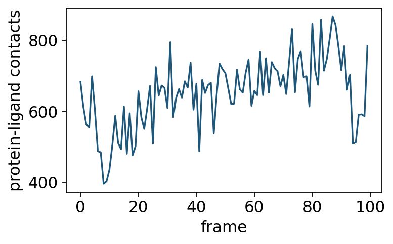
print(f'contacts: first {n_contacts[0]}, mean {n_contacts.mean():.0f}, last {n_contacts[-1]}')
contacts: first 683, mean 652, last 784
Finally, rescore over the ensemble with MM-GBSA:
decomposed into van der Waals, electrostatic, polar solvation (GBn2) and non-polar (surface-area) terms.
res = ov.mol.mmgbsa(cplx, frames=20)
res
OpenMM platform: CUDA (precision=mixed)
scoring 20 of 100 frames (GBn2 implicit solvent)
dG = -39.50 +/- 1.11 kcal/mol (vdW -45.5, elec -10.9, polar 24.1, nonpolar -7.2)
MMGBSAResult(dG = -39.50 +/- 1.11 kcal/mol, 20 frames)
res.to_frame().round(2)
| dG_kcal_mol | std | sem | n_frames | vdw_kcal_mol | electrostatic_kcal_mol | polar_solvation_kcal_mol | nonpolar_solvation_kcal_mol | |
|---|---|---|---|---|---|---|---|---|
| 0 | -39.5 | 4.97 | 1.11 | 20 | -45.48 | -10.91 | 24.06 | -7.18 |
Interpretation#
The fold is stable. RMSD plateaus around 0.15 nm, Rg holds at the literature value (~1.17 nm), and the secondary structure survives — this model can carry downstream work.
Flexibility is where biology says it should be. The RMSF peak is the C-terminal Gly-Gly tail that ubiquitin uses for conjugation. A prediction confidence score cannot tell you that; dynamics can.
Reading the MM-GBSA number honestly. End-point MM-GBSA is a relative ranking tool, not an experimental binding free energy:
it systematically overestimates affinity, often by 5–20 kcal/mol;
it includes no entropy term;
it uses implicit solvent, so bridging waters are invisible.
Use it to rank a congeneric series against itself, and always quote the spread
(res.sem) with the mean. For rigorous absolute free energies you need
alchemical FEP/TI — ov.mol.alchemical_free_energy documents why that is a
much more expensive undertaking and is deliberately not implemented here.
What you have gained over plain docking is real: the pose was relaxed in a force field with a thermostat, you can see whether it stayed bound, and the score is an ensemble average rather than one rigid snapshot.
Reproducibility. seed controls every stochastic step — hydrogen
placement, water and ion positions, initial velocities, thermostat and
barostat. Given the same MDSystem, seed, platform and precision, a run
repeats bit-for-bit. Across different platforms or precisions trajectories
diverge, because MD is chaotic; compare ensemble properties, not individual
frames. Every result object carries a provenance dict (engine versions,
forcefield, integrator, seed, platform, file hashes).
Next steps. ov.mol.production writes checkpoints — continue a run with
resume=traj.checkpoint. For a different target, everything here works
unchanged on an AlphaFold model from ov.mol.predict_structure.