Batch correction with Scanorama#
Scanorama (Hie, Bryson & Berger, Nat Biotechnol 2019) finds mutually-nearest-neighbours between batches and uses them to panorama-stitch the batches into a shared low-dimensional space. Strong when cell-type compositions differ across batches.
This is one of the omicverse batch-correction zoo tutorials. See batch/index for the overview / decision tree, or ../t_single_batch for the side-by-side comparison of every backend on a real benchmark.
Load a 2-batch demo from pbmc3k#
We use the canonical 10x pbmc3k dataset and synthesise a 2-batch label by random assignment, then plant a gene-shift on batch_B so the uncorrected UMAP shows a visible batch effect. This keeps the notebook self-contained and fast (~2 min end-to-end) — for a real multi-donor benchmark with [scib-metrics] scoring, see ../t_single_batch.
import omicverse as ov
ov.style()
import anndata as ad
import numpy as np
import pandas as pd

# NeurIPS 2021 multimodal hematopoiesis dataset — 3 real donor batches
# (s1d3, s2d1, s3d7), pre-annotated `cell_type` and raw `layers['counts']`.
# Same datasets used by the overview notebook ../t_single_batch.ipynb.
adata1 = ov.datasets.get_adata(
    'https://figshare.com/ndownloader/files/41932005',
    filename='neurips2021_s1d3.h5ad',
)
adata2 = ov.datasets.get_adata(
    'https://figshare.com/ndownloader/files/41932008',
    filename='neurips2021_s2d1.h5ad',
)
adata3 = ov.datasets.get_adata(
    'https://figshare.com/ndownloader/files/41932011',
    filename='neurips2021_s3d7.h5ad',
)
adata = ad.concat([adata1, adata2, adata3], merge='same')
adata.var_names_make_unique()
adata.obs_names_make_unique()
adata.obs['batch'] = adata.obs['batch'].astype('category')

# Subsample to a quick-running ~6 000 cells × 3 batches so the CPU
# backends (harmony / combat / scanorama / cca) finish in well under a
# minute. Drop this line for a full-resolution run.
_rng = np.random.default_rng(0)
_sel = _rng.choice(adata.n_obs, 6000, replace=False)
adata = adata[_sel].copy()
adata
🔬 Starting plot initialization...
🧬 Detecting GPU devices…
✅ NVIDIA CUDA GPUs detected: 1
    • [CUDA 0] NVIDIA H100 80GB HBM3
      Memory: 79.1 GB | Compute: 9.0

   ____            _     _    __
  / __ \____ ___  (_)___| |  / /__  _____________
 / / / / __ `__ \/ / ___/ | / / _ \/ ___/ ___/ _ \
/ /_/ / / / / / / / /__ | |/ /  __/ /  (__  )  __/
\____/_/ /_/ /_/_/\___/ |___/\___/_/  /____/\___/

🔖 Version: 2.2.1rc1   📚 Tutorials: https://omicverse.readthedocs.io/
✅ plot_set complete.

⚠️ File ./data/neurips2021_s1d3.h5ad already exists
 Loading data from ./data/neurips2021_s1d3.h5ad
✅ Successfully loaded: 5935 cells × 13953 genes
⚠️ File ./data/neurips2021_s2d1.h5ad already exists
 Loading data from ./data/neurips2021_s2d1.h5ad
✅ Successfully loaded: 10258 cells × 13953 genes
⚠️ File ./data/neurips2021_s3d7.h5ad already exists
 Loading data from ./data/neurips2021_s3d7.h5ad
✅ Successfully loaded: 11230 cells × 13953 genes
AnnData object with n_obs × n_vars = 6000 × 13953
    obs: 'GEX_n_genes_by_counts', 'GEX_pct_counts_mt', 'GEX_size_factors', 'GEX_phase', 'ADT_n_antibodies_by_counts', 'ADT_total_counts', 'ADT_iso_count', 'cell_type', 'batch', 'ADT_pseudotime_order', 'GEX_pseudotime_order', 'Samplename', 'Site', 'DonorNumber', 'Modality', 'VendorLot', 'DonorID', 'DonorAge', 'DonorBMI', 'DonorBloodType', 'DonorRace', 'Ethnicity', 'DonorGender', 'QCMeds', 'DonorSmoker', 'is_train'
    var: 'feature_types', 'gene_id'
    obsm: 'ADT_X_pca', 'ADT_X_umap', 'ADT_isotype_controls', 'GEX_X_pca', 'GEX_X_umap'
    layers: 'counts'
Preprocess + PCA + cluster#
Same QC → HVG-pearson → log-norm → PCA pipeline shared across every backend in the zoo. A quick Leiden cluster gives a synthetic celltype label that scANVI / scPoli can use as a prototype anchor.
# Standard omicverse preprocess (QC → HVG-via-pearson → log-norm → PCA).
# QC thresholds are loose because the NeurIPS data is already filtered.
adata = ov.pp.qc(adata, tresh={'mito_perc': 0.2, 'nUMIs': 200,
                                 'detected_genes': 100})
ov.utils.store_layers(adata, layers='counts')
adata = ov.pp.preprocess(adata, mode='shiftlog|pearson', n_HVGs=2000,
                         batch_key=None)
adata.raw = adata
adata = adata[:, adata.var.highly_variable_features].copy()
ov.pp.scale(adata)
ov.pp.pca(adata, layer='scaled', n_pcs=30)

# Neighbours graph for the pre-correction UMAP.
ov.pp.neighbors(adata, use_rep='scaled|original|X_pca', n_neighbors=15)

# The NeurIPS adata already carries a real `cell_type` annotation —
# rename it to `celltype` for the wrapper's expected schema. No Leiden
# needed; the labels are pre-annotated by the dataset authors.
adata.obs['celltype'] = adata.obs['cell_type'].astype('category')
adata
🖥️ Using CPU mode for QC...
   Auto-detected mitochondrial prefix: 'MT-'

📊 Step 1: Calculating QC Metrics

   ✓ Gene Family Detection:
   ┌──────────────────────────────┬────────────────────┬────────────────────┐
   │ Gene Family                  │ Genes Found        │ Detection Method   │
   ├──────────────────────────────┼────────────────────┼────────────────────┤
   │ Mitochondrial                │ 13                 │ Auto (MT-)         │
   ├──────────────────────────────┼────────────────────┼────────────────────┤
   │ Ribosomal                    │ 94                 │ Auto (RPS/RPL)     │
   ├──────────────────────────────┼────────────────────┼────────────────────┤
   │ Hemoglobin                   │ 11                 │ Auto (regex)       │
   └──────────────────────────────┴────────────────────┴────────────────────┘

   ✓ QC Metrics Summary:
   ┌─────────────────────────┬────────────────────┬─────────────────────────┐
   │ Metric                  │ Mean               │ Range (Min - Max)       │
   ├─────────────────────────┼────────────────────┼─────────────────────────┤
   │ nUMIs                   │ 20693              │ 1999 - 627052           │
   ├─────────────────────────┼────────────────────┼─────────────────────────┤
   │ Detected Genes          │ 1346               │ 104 - 5543              │
   ├─────────────────────────┼────────────────────┼─────────────────────────┤
   │ Mitochondrial %         │ 6.6%               │ 0.0% - 20.0%            │
   ├─────────────────────────┼────────────────────┼─────────────────────────┤
   │ Ribosomal %             │ 24.5%              │ 0.1% - 63.4%            │
   ├─────────────────────────┼────────────────────┼─────────────────────────┤
   │ Hemoglobin %            │ 10.1%              │ 0.0% - 96.1%            │
   └─────────────────────────┴────────────────────┴─────────────────────────┘

   📈 Original cell count: 6,000

🔧 Step 2: Quality Filtering (SEURAT)
   Thresholds: mito≤0.2, nUMIs≥200, genes≥100
   📊 Seurat Filter Results:
     • nUMIs filter (≥200): 0 cells failed (0.0%)
     • Genes filter (≥100): 0 cells failed (0.0%)
     • Mitochondrial filter (≤0.2): 1 cells failed (0.0%)
   ✓ Filters applied successfully
   ✓ Combined QC filters: 1 cells removed (0.0%)

🎯 Step 3: Final Filtering
   Parameters: min_genes=200, min_cells=3
   Ratios: max_genes_ratio=1, max_cells_ratio=1
✓ Final filtering: 44 cells, 0 genes removed

🔍 Step 4: Doublet Detection
   💡 Running pyscdblfinder (Python port of R scDblFinder)
   🔍 Running scdblfinder detection...
[ScDblFinder] wrote scDblFinder_score + scDblFinder_class — threshold=0.040
   ✓ scDblFinder completed: 169 doublets removed (2.8%)

╭─ SUMMARY: qc ──────────────────────────────────────────────────────╮
│  Duration: 27.5674s                                                │
│  Shape:    6,000 x 13,953 (Unchanged)                              │
│                                                                    │
│  CHANGES DETECTED                                                  │
│  ────────────────                                                  │
│  ● OBS    │ ✚ cell_complexity (float)                              │
│           │ ✚ detected_genes (int)                                 │
│           │ ✚ hb_perc (float)                                      │
│           │ ✚ mito_perc (float)                                    │
│           │ ✚ nUMIs (float)                                        │
│           │ ✚ n_counts (float)                                     │
│           │ ✚ n_genes (int)                                        │
│           │ ✚ n_genes_by_counts (int)                              │
│           │ ✚ passing_mt (bool)                                    │
│           │ ✚ passing_nUMIs (bool)                                 │
│           │ ✚ passing_ngenes (bool)                                │
│           │ ✚ pct_counts_hb (float)                                │
│           │ ✚ pct_counts_mt (float)                                │
│           │ ✚ pct_counts_ribo (float)                              │
│           │ ✚ ribo_perc (float)                                    │
│           │ ✚ total_counts (float)                                 │
│                                                                    │
│  ● VAR    │ ✚ hb (bool)                                            │
│           │ ✚ mt (bool)                                            │
│           │ ✚ ribo (bool)                                          │
│                                                                    │
╰────────────────────────────────────────────────────────────────────╯
......The X of adata have been stored in counts
🔍 [2026-05-29 04:55:22] Running preprocessing in 'cpu' mode...
Begin robust gene identification
    After filtration, 13953/13953 genes are kept.
    Among 13953 genes, 13953 genes are robust.
✅ Robust gene identification completed successfully.
Begin size normalization: shiftlog and HVGs selection pearson

🔍 Count Normalization:
   Target sum: 500000.0
   Exclude highly expressed: True
   Max fraction threshold: 0.2
⚠️ Excluding 6 highly-expressed genes from normalization computation
   Excluded genes: ['IGKC', 'HBB', 'MALAT1', 'HBA2', 'IGLC2', 'IGLC3']

✅ Count Normalization Completed Successfully!
   ✓ Processed: 5,786 cells × 13,953 genes
   ✓ Runtime: 0.26s

🔍 Highly Variable Genes Selection (Experimental):
   Method: pearson_residuals
   Target genes: 2,000
   Theta (overdispersion): 100
✅ Experimental HVG Selection Completed Successfully!
   ✓ Selected: 2,000 highly variable genes out of 13,953 total (14.3%)
   ✓ Results added to AnnData object:
     • 'highly_variable': Boolean vector (adata.var)
     • 'highly_variable_rank': Float vector (adata.var)
     • 'highly_variable_nbatches': Int vector (adata.var)
     • 'highly_variable_intersection': Boolean vector (adata.var)
     • 'means': Float vector (adata.var)
     • 'variances': Float vector (adata.var)
     • 'residual_variances': Float vector (adata.var)
    Time to analyze data in cpu: 1.92 seconds.
✅ Preprocessing completed successfully.
    Added:
        'highly_variable_features', boolean vector (adata.var)
        'means', float vector (adata.var)
        'variances', float vector (adata.var)
        'residual_variances', float vector (adata.var)
        'counts', raw counts layer (adata.layers)
    End of size normalization: shiftlog and HVGs selection pearson

╭─ SUMMARY: preprocess ──────────────────────────────────────────────╮
│  Duration: 2.1022s                                                 │
│  Shape:    5,786 x 13,953 (Unchanged)                              │
│                                                                    │
│  CHANGES DETECTED                                                  │
│  ────────────────                                                  │
│  ● VAR    │ ✚ highly_variable (bool)                               │
│           │ ✚ highly_variable_features (bool)                      │
│           │ ✚ highly_variable_rank (float)                         │
│           │ ✚ means (float)                                        │
│           │ ✚ n_cells (int)                                        │
│           │ ✚ percent_cells (float)                                │
│           │ ✚ residual_variances (float)                           │
│           │ ✚ robust (bool)                                        │
│           │ ✚ variances (float)                                    │
│                                                                    │
│  ● UNS    │ ✚ history_log                                          │
│           │ ✚ hvg                                                  │
│           │ ✚ log1p                                                │
│                                                                    │
╰────────────────────────────────────────────────────────────────────╯
╭─ SUMMARY: scale ───────────────────────────────────────────────────╮
│  Duration: 0.1537s                                                 │
│  Shape:    5,786 x 2,000 (Unchanged)                               │
│                                                                    │
│  CHANGES DETECTED                                                  │
│  ────────────────                                                  │
│  ● LAYERS │ ✚ scaled (array, 5786x2000)                            │
│                                                                    │
╰────────────────────────────────────────────────────────────────────╯
computing PCA🔍
    with n_comps=30
   🖥️ Using sklearn PCA for CPU computation
   🖥️ sklearn PCA backend: CPU computation
   📊 PCA input data type: ArrayView, shape: (5786, 2000), dtype: float64
🔧 PCA solver used: covariance_eigh
    finished✅ (1.17s)

╭─ SUMMARY: pca ─────────────────────────────────────────────────────╮
│  Duration: 1.169s                                                  │
│  Shape:    5,786 x 2,000 (Unchanged)                               │
│                                                                    │
│  CHANGES DETECTED                                                  │
│  ────────────────                                                  │
│  ● UNS    │ ✚ pca                                                  │
│           │ └─ params: {'zero_center': True, 'use_highly_variable': Tr...│
│           │ ✚ scaled|original|cum_sum_eigenvalues                  │
│           │ ✚ scaled|original|pca_var_ratios                       │
│                                                                    │
│  ● OBSM   │ ✚ X_pca (array, 5786x30)                               │
│           │ ✚ scaled|original|X_pca (array, 5786x30)               │
│                                                                    │
╰────────────────────────────────────────────────────────────────────╯
🖥️ Using Scanpy CPU to calculate neighbors...

🔍 K-Nearest Neighbors Graph Construction:
   Mode: cpu
   Neighbors: 15
   Method: umap
   Metric: euclidean
   Representation: scaled|original|X_pca
   🔍 Computing neighbor distances...
   🔍 Computing connectivity matrix...
   💡 Using UMAP-style connectivity
✓ Graph is fully connected

✅ KNN Graph Construction Completed Successfully!
   ✓ Processed: 5,786 cells with 15 neighbors each
   ✓ Results added to AnnData object:
     • 'neighbors': Neighbors metadata (adata.uns)
     • 'distances': Distance matrix (adata.obsp)
     • 'connectivities': Connectivity matrix (adata.obsp)

╭─ SUMMARY: neighbors ───────────────────────────────────────────────╮
│  Duration: 7.8732s                                                 │
│  Shape:    5,786 x 2,000 (Unchanged)                               │
│                                                                    │
│  CHANGES DETECTED                                                  │
│  ────────────────                                                  │
│  ● UNS    │ ✚ neighbors                                            │
│           │ └─ params: {'n_neighbors': 15, 'method': 'umap', 'random_s...│
│                                                                    │
│  ● OBSP   │ ✚ connectivities (sparse matrix, 5786x5786)            │
│           │ ✚ distances (sparse matrix, 5786x5786)                 │
│                                                                    │
╰────────────────────────────────────────────────────────────────────╯
AnnData object with n_obs × n_vars = 5786 × 2000
    obs: 'GEX_n_genes_by_counts', 'GEX_pct_counts_mt', 'GEX_size_factors', 'GEX_phase', 'ADT_n_antibodies_by_counts', 'ADT_total_counts', 'ADT_iso_count', 'cell_type', 'batch', 'ADT_pseudotime_order', 'GEX_pseudotime_order', 'Samplename', 'Site', 'DonorNumber', 'Modality', 'VendorLot', 'DonorID', 'DonorAge', 'DonorBMI', 'DonorBloodType', 'DonorRace', 'Ethnicity', 'DonorGender', 'QCMeds', 'DonorSmoker', 'is_train', 'nUMIs', 'mito_perc', 'ribo_perc', 'hb_perc', 'detected_genes', 'cell_complexity', 'n_counts', 'total_counts', 'n_genes', 'n_genes_by_counts', 'pct_counts_mt', 'pct_counts_ribo', 'pct_counts_hb', 'passing_mt', 'passing_nUMIs', 'passing_ngenes', 'predicted_doublet', 'doublet_score', 'scdblfinder_doublet', 'scdblfinder_score', 'celltype'
    var: 'feature_types', 'gene_id', 'mt', 'ribo', 'hb', 'n_cells', 'percent_cells', 'robust', 'highly_variable_features', 'means', 'variances', 'residual_variances', 'highly_variable_rank', 'highly_variable'
    uns: 'status', 'status_args', 'REFERENCE_MANU', '_ov_provenance', 'layers_counts', 'history_log', 'log1p', 'hvg', 'pca', 'scaled|original|pca_var_ratios', 'scaled|original|cum_sum_eigenvalues', 'neighbors'
    obsm: 'ADT_X_pca', 'ADT_X_umap', 'ADT_isotype_controls', 'GEX_X_pca', 'GEX_X_umap', 'X_pca', 'scaled|original|X_pca'
    varm: 'PCs', 'scaled|original|pca_loadings'
    layers: 'counts', 'scaled'
    obsp: 'distances', 'connectivities'
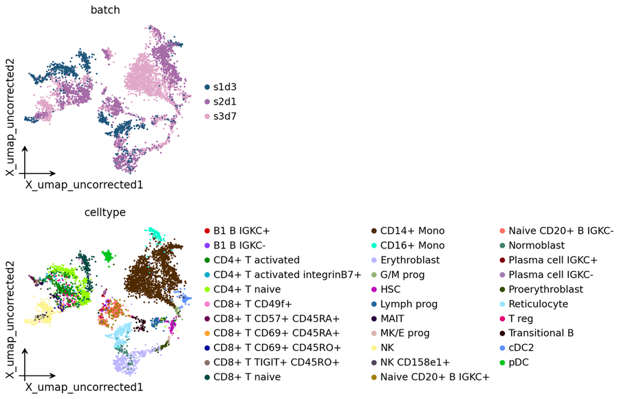
Uncorrected baseline#
The planted batch effect is visible in the uncorrected UMAP:
# Pre-correction UMAP shows the planted batch effect.
ov.pp.umap(adata, min_dist=0.3)
adata.obsm['X_umap_uncorrected'] = adata.obsm['X_umap'].copy()
ov.pl.embedding(adata, basis='X_umap_uncorrected',
                color=['batch', 'celltype'],
                frameon='small', wspace=0.5)
🔍 [2026-05-29 04:55:34] Running UMAP in 'cpu' mode...
🖥️ Using Scanpy CPU UMAP...

🔍 UMAP Dimensionality Reduction:
   Mode: cpu
   Method: umap
   Components: 2
   Min distance: 0.3
{'n_neighbors': 15, 'method': 'umap', 'random_state': 0, 'metric': 'euclidean', 'use_rep': 'scaled|original|X_pca'}
   🔍 Computing UMAP parameters...
   🔍 Computing UMAP embedding (classic method)...
✅ UMAP Dimensionality Reduction Completed Successfully!
   ✓ Embedding shape: 5,786 cells × 2 dimensions
   ✓ Results added to AnnData object:
     • 'X_umap': UMAP coordinates (adata.obsm)
     • 'umap': UMAP parameters (adata.uns)
✅ UMAP completed successfully.

╭─ SUMMARY: umap ────────────────────────────────────────────────────╮
│  Duration: 0.933s                                                  │
│  Shape:    5,786 x 2,000 (Unchanged)                               │
│                                                                    │
│  CHANGES DETECTED                                                  │
│  ────────────────                                                  │
│  ● UNS    │ ✚ umap                                                 │
│           │ └─ params: {'a': np.float64(0.9921756195894755), 'b': np.f...│
│                                                                    │
│  ● OBSM   │ ✚ X_umap (array, 5786x2)                               │
│                                                                    │
╰────────────────────────────────────────────────────────────────────╯
Run ov.single.batch_correction(methods='scanorama')#
For the scvi-tools family backends, the wrapper auto-routes **kwargs between the model’s __init__ (architecture) and .train() (optimisation) destinations. See the Key parameters section below.
ov.single.batch_correction(
    adata,
    batch_key='batch',
    methods='scanorama',
    n_pcs=30,
)
...Begin using scanorama to correct batch effect
s1d3
s2d1
s3d7
Found 2000 genes among all datasets
[[0.         0.61416667 0.63      ]
 [0.         0.         0.83050847]
 [0.         0.         0.        ]]
Processing datasets (1, 2)
Processing datasets (0, 2)
Processing datasets (0, 1)
(5786, 30)

╭─ SUMMARY: batch_correction ────────────────────────────────────────╮
│  Duration: 2.1483s                                                 │
│  Shape:    5,786 x 2,000 (Unchanged)                               │
│                                                                    │
│  CHANGES DETECTED                                                  │
│  ────────────────                                                  │
│  ● OBSM   │ ✚ X_scanorama (array, 5786x30)                         │
│                                                                    │
╰────────────────────────────────────────────────────────────────────╯
AnnData object with n_obs × n_vars = 5786 × 2000
    obs: 'GEX_n_genes_by_counts', 'GEX_pct_counts_mt', 'GEX_size_factors', 'GEX_phase', 'ADT_n_antibodies_by_counts', 'ADT_total_counts', 'ADT_iso_count', 'cell_type', 'batch', 'ADT_pseudotime_order', 'GEX_pseudotime_order', 'Samplename', 'Site', 'DonorNumber', 'Modality', 'VendorLot', 'DonorID', 'DonorAge', 'DonorBMI', 'DonorBloodType', 'DonorRace', 'Ethnicity', 'DonorGender', 'QCMeds', 'DonorSmoker', 'is_train', 'nUMIs', 'mito_perc', 'ribo_perc', 'hb_perc', 'detected_genes', 'cell_complexity', 'n_counts', 'total_counts', 'n_genes', 'n_genes_by_counts', 'pct_counts_mt', 'pct_counts_ribo', 'pct_counts_hb', 'passing_mt', 'passing_nUMIs', 'passing_ngenes', 'predicted_doublet', 'doublet_score', 'scdblfinder_doublet', 'scdblfinder_score', 'celltype'
    var: 'feature_types', 'gene_id', 'mt', 'ribo', 'hb', 'n_cells', 'percent_cells', 'robust', 'highly_variable_features', 'means', 'variances', 'residual_variances', 'highly_variable_rank', 'highly_variable'
    uns: 'status', 'status_args', 'REFERENCE_MANU', '_ov_provenance', 'layers_counts', 'history_log', 'log1p', 'hvg', 'pca', 'scaled|original|pca_var_ratios', 'scaled|original|cum_sum_eigenvalues', 'neighbors', 'umap', 'batch_colors_rgba', 'batch_colors', 'celltype_colors_rgba', 'celltype_colors'
    obsm: 'ADT_X_pca', 'ADT_X_umap', 'ADT_isotype_controls', 'GEX_X_pca', 'GEX_X_umap', 'X_pca', 'scaled|original|X_pca', 'X_umap', 'X_umap_uncorrected', 'X_scanorama'
    varm: 'PCs', 'scaled|original|pca_loadings'
    layers: 'counts', 'scaled'
    obsp: 'distances', 'connectivities'
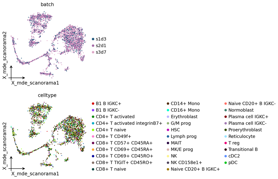
Corrected embedding#
Every backend writes its corrected representation to a stable obsm key — for this one it is adata.obsm['X_scanorama']. We project via ov.utils.mde for a lightweight UMAP-style display.
adata.obsm['X_mde_scanorama'] = ov.utils.mde(adata.obsm['X_scanorama'])
ov.pl.embedding(
    adata,
    basis='X_mde_scanorama',
    color=['batch', 'celltype'],
    frameon='small',
    wspace=0.5,
)
Key parameters#
n_pcs— embedding dimension (default 50).Internally requires raw counts in
.Xfor some operations — the wrapper handles the routing.