Trajectory Inference with SCORPIUS#
SCORPIUS (Cannoodt 2016) is a linear-trajectory backend: it reduces the cells to a 1-D principal curve and reports each cell’s distance along that curve. There are no branch labels — pick SCORPIUS when biology says the differentiation is unbranched, or as a fast first pass before deciding which branching method to use.
Backend: pyscorpius — Python port of R dynverse/SCORPIUS.
Install#
pip install omicverse[trajectory]
import numpy as np
import matplotlib.pyplot as plt
import warnings
warnings.filterwarnings("ignore", category=FutureWarning)

import omicverse as ov
ov.plot_set(font_path='Arial')

%load_ext autoreload
%autoreload 2
🔬 Starting plot initialization...
Using already downloaded Arial font from: /tmp/omicverse_arial.ttf
Registered as: Arial
🧬 Detecting GPU devices…
✅ NVIDIA CUDA GPUs detected: 1
    • [CUDA 0] NVIDIA H100 80GB HBM3
      Memory: 79.1 GB | Compute: 9.0

   ____            _     _    __
  / __ \____ ___  (_)___| |  / /__  _____________
 / / / / __ `__ \/ / ___/ | / / _ \/ ___/ ___/ _ \
/ /_/ / / / / / / / /__ | |/ /  __/ /  (__  )  __/
\____/_/ /_/ /_/_/\___/ |___/\___/_/  /____/\___/

🔖 Version: 2.2.1rc1   📚 Tutorials: https://omicverse.readthedocs.io/
✅ plot_set complete.
adata = ov.datasets.pancreatic_endocrinogenesis()
⚠️ File ./data/endocrinogenesis_day15.h5ad already exists
 Loading data from ./data/endocrinogenesis_day15.h5ad
✅ Successfully loaded: 3696 cells × 27998 genes
adata = ov.pp.preprocess(adata, mode='shiftlog|pearson', n_HVGs=3000)
adata.raw = adata
adata = adata[:, adata.var.highly_variable_features]
ov.pp.scale(adata)
ov.pp.pca(adata, layer='scaled', n_pcs=50)
🔍 [2026-05-25 02:35:01] Running preprocessing in 'cpu' mode...
Begin robust gene identification
    After filtration, 17750/27998 genes are kept.
    Among 17750 genes, 16426 genes are robust.
✅ Robust gene identification completed successfully.
Begin size normalization: shiftlog and HVGs selection pearson
🔍 Count Normalization:
   Target sum: 500000.0
   Exclude highly expressed: True
   Max fraction threshold: 0.2
   ⚠️ Excluding 1 highly-expressed genes from normalization computation
   Excluded genes: ['Ghrl']
✅ Count Normalization Completed Successfully!
   ✓ Processed: 3,696 cells × 16,426 genes
   ✓ Runtime: 0.26s

🔍 Highly Variable Genes Selection (Experimental):
   Method: pearson_residuals
   Target genes: 3,000
   Theta (overdispersion): 100
✅ Experimental HVG Selection Completed Successfully!
   ✓ Selected: 3,000 highly variable genes out of 16,426 total (18.3%)
   ✓ Results added to AnnData object:
     • 'highly_variable': Boolean vector (adata.var)
     • 'highly_variable_rank': Float vector (adata.var)
     • 'highly_variable_nbatches': Int vector (adata.var)
     • 'highly_variable_intersection': Boolean vector (adata.var)
     • 'means': Float vector (adata.var)
     • 'variances': Float vector (adata.var)
     • 'residual_variances': Float vector (adata.var)
    Time to analyze data in cpu: 2.17 seconds.
✅ Preprocessing completed successfully.
    Added:
        'highly_variable_features', boolean vector (adata.var)
        'means', float vector (adata.var)
        'variances', float vector (adata.var)
        'residual_variances', float vector (adata.var)
        'counts', raw counts layer (adata.layers)
    End of size normalization: shiftlog and HVGs selection pearson

╭─ SUMMARY: preprocess ──────────────────────────────────────────────╮
│  Duration: 2.5622s                                                 │
│  Shape:    3,696 x 27,998 -> 3,696 x 16,426                        │
│                                                                    │
│  CHANGES DETECTED                                                  │
│  ────────────────                                                  │
│  ● VAR    │ ✚ highly_variable (bool)                               │
│           │ ✚ highly_variable_features (bool)                      │
│           │ ✚ highly_variable_rank (float)                         │
│           │ ✚ means (float)                                        │
│           │ ✚ n_cells (int)                                        │
│           │ ✚ percent_cells (float)                                │
│           │ ✚ residual_variances (float)                           │
│           │ ✚ robust (bool)                                        │
│           │ ✚ variances (float)                                    │
│                                                                    │
│  ● UNS    │ ✚ REFERENCE_MANU                                       │
│           │ ✚ _ov_provenance                                       │
│           │ ✚ history_log                                          │
│           │ ✚ hvg                                                  │
│           │ ✚ log1p                                                │
│           │ ✚ status                                               │
│           │ ✚ status_args                                          │
│                                                                    │
│  ● LAYERS │ ✚ counts (sparse matrix, 3696x16426)                   │
│                                                                    │
╰────────────────────────────────────────────────────────────────────╯
╭─ SUMMARY: scale ───────────────────────────────────────────────────╮
│  Duration: 0.7502s                                                 │
│  Shape:    3,696 x 3,000 (Unchanged)                               │
│                                                                    │
│  CHANGES DETECTED                                                  │
│  ────────────────                                                  │
│  ● LAYERS │ ✚ scaled (array, 3696x3000)                            │
│                                                                    │
╰────────────────────────────────────────────────────────────────────╯
computing PCA🔍
    with n_comps=50
   🖥️ Using sklearn PCA for CPU computation
   🖥️ sklearn PCA backend: CPU computation
   📊 PCA input data type: ArrayView, shape: (3696, 3000), dtype: float64
🔧 PCA solver used: covariance_eigh
    finished✅ (11.51s)

╭─ SUMMARY: pca ─────────────────────────────────────────────────────╮
│  Duration: 11.5234s                                                │
│  Shape:    3,696 x 3,000 (Unchanged)                               │
│                                                                    │
│  CHANGES DETECTED                                                  │
│  ────────────────                                                  │
│  ● UNS    │ ✚ scaled|original|cum_sum_eigenvalues                  │
│           │ ✚ scaled|original|pca_var_ratios                       │
│                                                                    │
│  ● OBSM   │ ✚ scaled|original|X_pca (array, 3696x50)               │
│                                                                    │
╰────────────────────────────────────────────────────────────────────╯
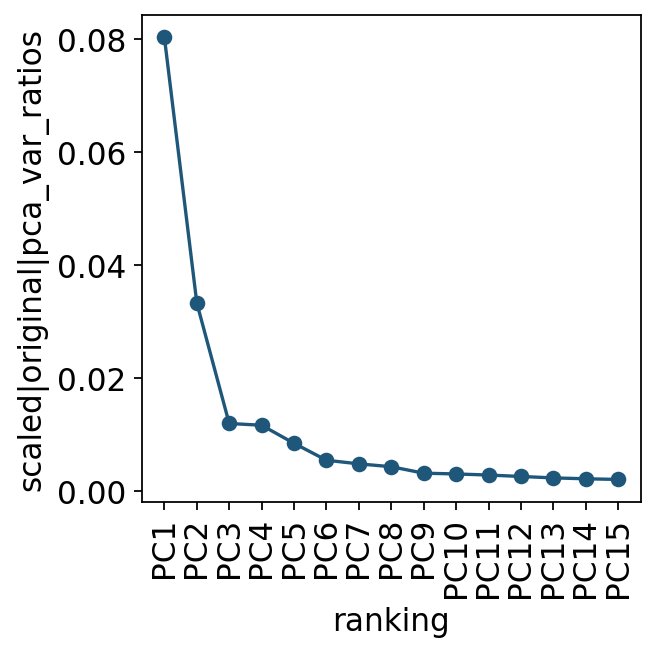
We first inspect the variance explained by principal components to choose a practical PC range for neighbour and graph computations.
ov.utils.plot_pca_variance_ratio(adata, n_pcs=15)
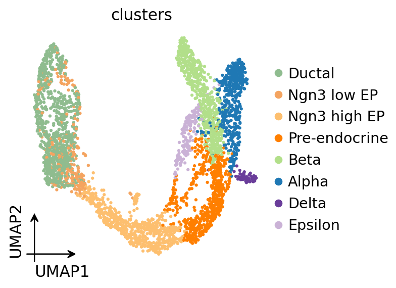
ov.pl.umap(
    adata,
    color='clusters'
)
X_umap converted to UMAP to visualize and saved to adata.obsm['UMAP']
if you want to use X_umap, please set convert=False
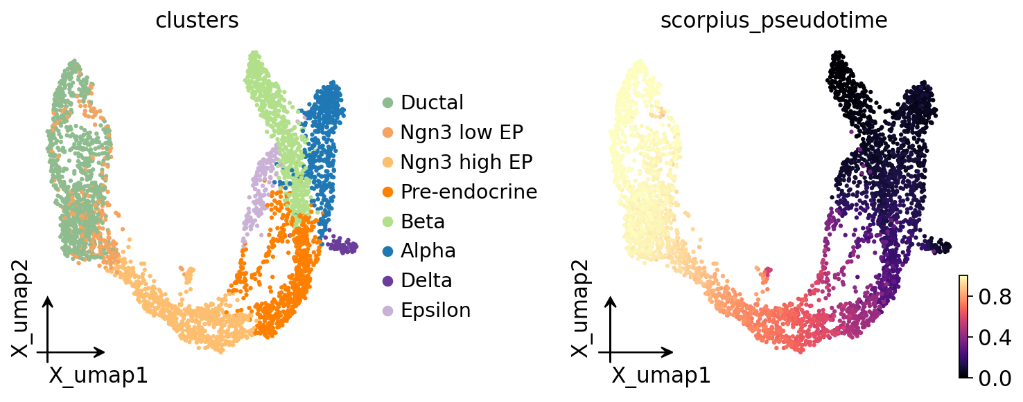
SCORPIUS#
Traj=ov.single.TrajInfer(
    adata,
    basis='X_umap',
    groupby='clusters',
    use_rep='scaled|original|X_pca',
    n_comps=50,
)
Traj.set_origin_cells('Ductal')
Traj.inference(method='scorpius', ndim=3)
Visualize pseudotime on UMAP#
ov.pl.embedding(
    adata, basis='X_umap',
    color=['clusters', 'scorpius_pseudotime'],
    frameon='small',
    cmap='magma',
)
Downstream notes#
SCORPIUS is linear by construction — there is no branch field to plot. If your topology might be branching, run 'tscan' / 'destiny' / 'slingshot' instead.
Reference#
Saelens W. et al. A comparison of single-cell trajectory inference methods. Nat Biotechnol 37, 547–554 (2019). doi:10.1038/s41587-019-0071-9
Recommended backend (Slingshot): t_traj_recommended
All zoo backends: zoo/index