Batch correction with totalVI (joint RNA + protein)#
totalVI (Gayoso et al., Nat Methods 2021) is scvi-tools’ joint generative model for CITE-seq / Total-seq data. It learns a shared latent space across RNA and ADT while explicitly modelling protein background, and corrects batch effects in both modalities. This demo synthesises an ADT matrix — on real data, populate adata.obsm['protein_counts'] with your (cell × protein) raw ADT counts before the call.
This is one of the omicverse batch-correction zoo tutorials. See batch/index for the overview / decision tree, or ../t_single_batch for the side-by-side comparison of every backend on a real benchmark.
Load a real CITE-seq 2-batch dataset#
We use scvi.data.pbmcs_10x_cite_seq — a Stoeckius-style 10x
PBMC CITE-seq dataset bundled with scvi-tools, 10 849 cells across
two real donor batches (PBMC10k + PBMC5k), 15 792 genes in .X
and 14 surface proteins in obsm['protein_expression']. The NeurIPS
2021 multimodal hematopoiesis dataset used by the other zoo
notebooks ships GEX-only on figshare, so for totalVI — which needs
real protein counts — we switch to this self-contained CITE-seq
demo. The pipeline is otherwise identical to the rest of the zoo.
import omicverse as ov
ov.style()
import anndata as ad
import numpy as np
import pandas as pd
import scvi.data as scvi_data
import os

# Real 10x PBMC CITE-seq — 2 batches, 15 792 genes, 14 ADT proteins
# in `obsm['protein_expression']`. Cached under ./data/scvi_cache so
# subsequent re-renders hit local disk.
os.makedirs('./data/scvi_cache', exist_ok=True)
adata = scvi_data.pbmcs_10x_cite_seq(save_path='./data/scvi_cache')
adata.obs_names_make_unique()
adata.var_names_make_unique()
adata.obs['batch'] = adata.obs['batch'].astype('category')

# Subsample to ~6 000 cells so the whole notebook stays GPU-snappy.
_rng = np.random.default_rng(0)
_sel = _rng.choice(adata.n_obs, 6000, replace=False)
adata = adata[_sel].copy()

# totalVI needs raw counts: layers['counts'] for genes + the protein
# matrix already lives in obsm['protein_expression'].
adata.layers['counts'] = adata.X.copy()
print(adata)
print('protein_expression shape:', adata.obsm['protein_expression'].shape)
🔬 Starting plot initialization...
🧬 Detecting GPU devices…
✅ NVIDIA CUDA GPUs detected: 1
    • [CUDA 0] NVIDIA H100 80GB HBM3
      Memory: 79.1 GB | Compute: 9.0

   ____            _     _    __
  / __ \____ ___  (_)___| |  / /__  _____________
 / / / / __ `__ \/ / ___/ | / / _ \/ ___/ ___/ _ \
/ /_/ / / / / / / / /__ | |/ /  __/ /  (__  )  __/
\____/_/ /_/ /_/_/\___/ |___/\___/_/  /____/\___/

🔖 Version: 2.2.1rc1   📚 Tutorials: https://omicverse.readthedocs.io/
✅ plot_set complete.
INFO     File ./data/scvi_cache/pbmc_10k_protein_v3.h5ad already downloaded
INFO     File ./data/scvi_cache/pbmc_5k_protein_v3.h5ad already downloaded
AnnData object with n_obs × n_vars = 6000 × 15792
    obs: 'n_genes', 'percent_mito', 'n_counts', 'batch'
    obsm: 'protein_expression'
    layers: 'counts'
protein_expression shape: (6000, 14)
Preprocess + PCA + cluster#
Same QC → HVG-via-pearson → log-norm → PCA pipeline shared across
every backend in the zoo. The pbmcs_10x_cite_seq dataset ships
without pre-annotated cell types, so we run a quick Leiden clustering
on the PCA neighbours graph for celltype colouring on the
uncorrected / corrected UMAP — the labels are for visualisation, not
input to totalVI.
# Standard omicverse preprocess (QC → HVG-via-pearson → log-norm → PCA).
adata = ov.pp.qc(adata, tresh={'mito_perc': 0.2, 'nUMIs': 200,
                                 'detected_genes': 100})
# layers['counts'] was set above to preserve the raw matrix; preprocess
# operates on .X, so it's safe to log-normalise and HVG-select here.
adata = ov.pp.preprocess(adata, mode='shiftlog|pearson', n_HVGs=2000,
                         batch_key=None)
adata.raw = adata
adata = adata[:, adata.var.highly_variable_features].copy()
ov.pp.scale(adata)
ov.pp.pca(adata, layer='scaled', n_pcs=30)
ov.pp.neighbors(adata, use_rep='scaled|original|X_pca', n_neighbors=15)

# Quick Leiden cluster as `celltype` for colour-only purposes —
# pbmcs_10x_cite_seq ships without pre-annotation. totalVI itself
# does not see these labels.
ov.pp.leiden(adata, resolution=0.5, key_added='celltype')
adata.obs['celltype'] = adata.obs['celltype'].astype('category')
adata
🖥️ Using CPU mode for QC...
   Auto-detected mitochondrial prefix: 'MT-'

📊 Step 1: Calculating QC Metrics

   ✓ Gene Family Detection:
   ┌──────────────────────────────┬────────────────────┬────────────────────┐
   │ Gene Family                  │ Genes Found        │ Detection Method   │
   ├──────────────────────────────┼────────────────────┼────────────────────┤
   │ Mitochondrial                │ 13                 │ Auto (MT-)         │
   ├──────────────────────────────┼────────────────────┼────────────────────┤
   │ Ribosomal                    │ 95                 │ Auto (RPS/RPL)     │
   ├──────────────────────────────┼────────────────────┼────────────────────┤
   │ Hemoglobin                   │ 6                  │ Auto (regex)       │
   └──────────────────────────────┴────────────────────┴────────────────────┘

   ✓ QC Metrics Summary:
   ┌─────────────────────────┬────────────────────┬─────────────────────────┐
   │ Metric                  │ Mean               │ Range (Min - Max)       │
   ├─────────────────────────┼────────────────────┼─────────────────────────┤
   │ nUMIs                   │ 5171               │ 516 - 19960             │
   ├─────────────────────────┼────────────────────┼─────────────────────────┤
   │ Detected Genes          │ 1685               │ 291 - 4360              │
   ├─────────────────────────┼────────────────────┼─────────────────────────┤
   │ Mitochondrial %         │ 6.9%               │ 0.8% - 20.0%            │
   ├─────────────────────────┼────────────────────┼─────────────────────────┤
   │ Ribosomal %             │ 27.5%              │ 0.8% - 54.7%            │
   ├─────────────────────────┼────────────────────┼─────────────────────────┤
   │ Hemoglobin %            │ 0.0%               │ 0.0% - 0.2%             │
   └─────────────────────────┴────────────────────┴─────────────────────────┘

   📈 Original cell count: 6,000

🔧 Step 2: Quality Filtering (SEURAT)
   Thresholds: mito≤0.2, nUMIs≥200, genes≥100
   📊 Seurat Filter Results:
     • nUMIs filter (≥200): 0 cells failed (0.0%)
     • Genes filter (≥100): 0 cells failed (0.0%)
     • Mitochondrial filter (≤0.2): 1 cells failed (0.0%)
   ✓ Filters applied successfully
   ✓ Combined QC filters: 1 cells removed (0.0%)

🎯 Step 3: Final Filtering
   Parameters: min_genes=200, min_cells=3
   Ratios: max_genes_ratio=1, max_cells_ratio=1
✓ Final filtering: 0 cells, 11 genes removed

🔍 Step 4: Doublet Detection
   💡 Running pyscdblfinder (Python port of R scDblFinder)
   🔍 Running scdblfinder detection...
[ScDblFinder] wrote scDblFinder_score + scDblFinder_class — threshold=0.060
   ✓ scDblFinder completed: 178 doublets removed (3.0%)
╭─ SUMMARY: qc ──────────────────────────────────────────────────────╮
│  Duration: 30.6914s                                                │
│  Shape:    6,000 x 15,792 (Unchanged)                              │
│                                                                    │
│  CHANGES DETECTED                                                  │
│  ────────────────                                                  │
│  ● OBS    │ ✚ cell_complexity (float)                              │
│           │ ✚ detected_genes (int)                                 │
│           │ ✚ hb_perc (float)                                      │
│           │ ✚ mito_perc (float)                                    │
│           │ ✚ nUMIs (float)                                        │
│           │ ✚ n_genes_by_counts (int)                              │
│           │ ✚ passing_mt (bool)                                    │
│           │ ✚ passing_nUMIs (bool)                                 │
│           │ ✚ passing_ngenes (bool)                                │
│           │ ✚ pct_counts_hb (float)                                │
│           │ ✚ pct_counts_mt (float)                                │
│           │ ✚ pct_counts_ribo (float)                              │
│           │ ✚ ribo_perc (float)                                    │
│           │ ✚ total_counts (float)                                 │
│                                                                    │
│  ● VAR    │ ✚ hb (bool)                                            │
│           │ ✚ mt (bool)                                            │
│           │ ✚ ribo (bool)                                          │
│                                                                    │
╰────────────────────────────────────────────────────────────────────╯
🔍 [2026-05-29 05:09:14] Running preprocessing in 'cpu' mode...
Begin robust gene identification
    After filtration, 15781/15781 genes are kept.
    Among 15781 genes, 15781 genes are robust.
✅ Robust gene identification completed successfully.
Begin size normalization: shiftlog and HVGs selection pearson
🔍 Count Normalization:
   Target sum: 500000.0
   Exclude highly expressed: True
   Max fraction threshold: 0.2
   ⚠️ Excluding 3 highly-expressed genes from normalization computation
   Excluded genes: ['IGKC', 'MALAT1', 'IGLC3']
✅ Count Normalization Completed Successfully!
   ✓ Processed: 5,821 cells × 15,781 genes
   ✓ Runtime: 0.84s

🔍 Highly Variable Genes Selection (Experimental):
   Method: pearson_residuals
   Target genes: 2,000
   Theta (overdispersion): 100
✅ Experimental HVG Selection Completed Successfully!
   ✓ Selected: 2,000 highly variable genes out of 15,781 total (12.7%)
   ✓ Results added to AnnData object:
     • 'highly_variable': Boolean vector (adata.var)
     • 'highly_variable_rank': Float vector (adata.var)
     • 'highly_variable_nbatches': Int vector (adata.var)
     • 'highly_variable_intersection': Boolean vector (adata.var)
     • 'means': Float vector (adata.var)
     • 'variances': Float vector (adata.var)
     • 'residual_variances': Float vector (adata.var)
    Time to analyze data in cpu: 7.22 seconds.
✅ Preprocessing completed successfully.
    Added:
        'highly_variable_features', boolean vector (adata.var)
        'means', float vector (adata.var)
        'variances', float vector (adata.var)
        'residual_variances', float vector (adata.var)
        'counts', raw counts layer (adata.layers)
    End of size normalization: shiftlog and HVGs selection pearson

╭─ SUMMARY: preprocess ──────────────────────────────────────────────╮
│  Duration: 7.4513s                                                 │
│  Shape:    5,821 x 15,781 (Unchanged)                              │
│                                                                    │
│  CHANGES DETECTED                                                  │
│  ────────────────                                                  │
│  ● VAR    │ ✚ highly_variable (bool)                               │
│           │ ✚ highly_variable_features (bool)                      │
│           │ ✚ highly_variable_rank (float)                         │
│           │ ✚ means (float)                                        │
│           │ ✚ residual_variances (float)                           │
│           │ ✚ robust (bool)                                        │
│           │ ✚ variances (float)                                    │
│                                                                    │
│  ● UNS    │ ✚ history_log                                          │
│           │ ✚ hvg                                                  │
│           │ ✚ log1p                                                │
│                                                                    │
╰────────────────────────────────────────────────────────────────────╯
╭─ SUMMARY: scale ───────────────────────────────────────────────────╮
│  Duration: 0.3267s                                                 │
│  Shape:    5,821 x 2,000 (Unchanged)                               │
│                                                                    │
│  CHANGES DETECTED                                                  │
│  ────────────────                                                  │
│  ● LAYERS │ ✚ scaled (array, 5821x2000)                            │
│                                                                    │
╰────────────────────────────────────────────────────────────────────╯
computing PCA🔍
    with n_comps=30
   🖥️ Using sklearn PCA for CPU computation
   🖥️ sklearn PCA backend: CPU computation
   📊 PCA input data type: ArrayView, shape: (5821, 2000), dtype: float32
🔧 PCA solver used: covariance_eigh
    finished✅ (1.18s)

╭─ SUMMARY: pca ─────────────────────────────────────────────────────╮
│  Duration: 1.1866s                                                 │
│  Shape:    5,821 x 2,000 (Unchanged)                               │
│                                                                    │
│  CHANGES DETECTED                                                  │
│  ────────────────                                                  │
│  ● UNS    │ ✚ pca                                                  │
│           │ └─ params: {'zero_center': True, 'use_highly_variable': Tr...│
│           │ ✚ scaled|original|cum_sum_eigenvalues                  │
│           │ ✚ scaled|original|pca_var_ratios                       │
│                                                                    │
│  ● OBSM   │ ✚ X_pca (array, 5821x30)                               │
│           │ ✚ scaled|original|X_pca (array, 5821x30)               │
│                                                                    │
╰────────────────────────────────────────────────────────────────────╯
🖥️ Using Scanpy CPU to calculate neighbors...

🔍 K-Nearest Neighbors Graph Construction:
   Mode: cpu
   Neighbors: 15
   Method: umap
   Metric: euclidean
   Representation: scaled|original|X_pca
   🔍 Computing neighbor distances...
   🔍 Computing connectivity matrix...
   💡 Using UMAP-style connectivity
✓ Graph is fully connected

✅ KNN Graph Construction Completed Successfully!
   ✓ Processed: 5,821 cells with 15 neighbors each
   ✓ Results added to AnnData object:
     • 'neighbors': Neighbors metadata (adata.uns)
     • 'distances': Distance matrix (adata.obsp)
     • 'connectivities': Connectivity matrix (adata.obsp)

╭─ SUMMARY: neighbors ───────────────────────────────────────────────╮
│  Duration: 8.0982s                                                 │
│  Shape:    5,821 x 2,000 (Unchanged)                               │
│                                                                    │
│  CHANGES DETECTED                                                  │
│  ────────────────                                                  │
│  ● UNS    │ ✚ neighbors                                            │
│           │ └─ params: {'n_neighbors': 15, 'method': 'umap', 'random_s...│
│                                                                    │
│  ● OBSP   │ ✚ connectivities (sparse matrix, 5821x5821)            │
│           │ ✚ distances (sparse matrix, 5821x5821)                 │
│                                                                    │
╰────────────────────────────────────────────────────────────────────╯
🖥️ Using Scanpy CPU Leiden...
running Leiden clustering
    finished (0.18s)
    found 15 clusters and added
    'celltype', the cluster labels (adata.obs, categorical)

╭─ SUMMARY: leiden ──────────────────────────────────────────────────╮
│  Duration: 0.1814s                                                 │
│  Shape:    5,821 x 2,000 (Unchanged)                               │
│                                                                    │
│  CHANGES DETECTED                                                  │
│  ────────────────                                                  │
│  ● OBS    │ ✚ celltype (category)                                  │
│           │ ✚ leiden (category)                                    │
│                                                                    │
│  ● UNS    │ ✚ celltype                                             │
│           │ └─ params: {'resolution': 0.5, 'random_state': 0, 'n_itera...│
│                                                                    │
╰────────────────────────────────────────────────────────────────────╯
AnnData object with n_obs × n_vars = 5821 × 2000
    obs: 'n_genes', 'percent_mito', 'n_counts', 'batch', 'nUMIs', 'mito_perc', 'ribo_perc', 'hb_perc', 'detected_genes', 'cell_complexity', 'total_counts', 'n_genes_by_counts', 'pct_counts_mt', 'pct_counts_ribo', 'pct_counts_hb', 'passing_mt', 'passing_nUMIs', 'passing_ngenes', 'predicted_doublet', 'doublet_score', 'scdblfinder_doublet', 'scdblfinder_score', 'celltype', 'leiden'
    var: 'mt', 'ribo', 'hb', 'robust', 'highly_variable_features', 'means', 'variances', 'residual_variances', 'highly_variable_rank', 'highly_variable'
    uns: 'status', 'status_args', 'REFERENCE_MANU', '_ov_provenance', 'history_log', 'log1p', 'hvg', 'pca', 'scaled|original|pca_var_ratios', 'scaled|original|cum_sum_eigenvalues', 'neighbors', 'celltype'
    obsm: 'protein_expression', 'X_pca', 'scaled|original|X_pca'
    varm: 'PCs', 'scaled|original|pca_loadings'
    layers: 'counts', 'scaled'
    obsp: 'distances', 'connectivities'
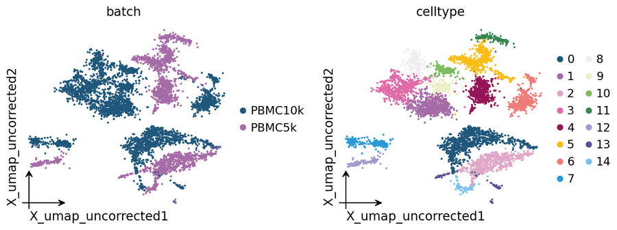
Uncorrected baseline#
The planted batch effect is visible in the uncorrected UMAP:
# Pre-correction UMAP shows the planted batch effect.
ov.pp.umap(adata, min_dist=0.3)
adata.obsm['X_umap_uncorrected'] = adata.obsm['X_umap'].copy()
ov.pl.embedding(adata, basis='X_umap_uncorrected',
                color=['batch', 'celltype'],
                frameon='small', wspace=0.5)
🔍 [2026-05-29 05:09:32] Running UMAP in 'cpu' mode...
🖥️ Using Scanpy CPU UMAP...
🔍 UMAP Dimensionality Reduction:
   Mode: cpu
   Method: umap
   Components: 2
   Min distance: 0.3
{'n_neighbors': 15, 'method': 'umap', 'random_state': 0, 'metric': 'euclidean', 'use_rep': 'scaled|original|X_pca'}
   🔍 Computing UMAP parameters...
   🔍 Computing UMAP embedding (classic method)...
✅ UMAP Dimensionality Reduction Completed Successfully!
   ✓ Embedding shape: 5,821 cells × 2 dimensions
   ✓ Results added to AnnData object:
     • 'X_umap': UMAP coordinates (adata.obsm)
     • 'umap': UMAP parameters (adata.uns)
✅ UMAP completed successfully.

╭─ SUMMARY: umap ────────────────────────────────────────────────────╮
│  Duration: 0.9007s                                                 │
│  Shape:    5,821 x 2,000 (Unchanged)                               │
│                                                                    │
│  CHANGES DETECTED                                                  │
│  ────────────────                                                  │
│  ● UNS    │ ✚ umap                                                 │
│           │ └─ params: {'a': np.float64(0.9921756195894755), 'b': np.f...│
│                                                                    │
│  ● OBSM   │ ✚ X_umap (array, 5821x2)                               │
│                                                                    │
╰────────────────────────────────────────────────────────────────────╯
Run ov.single.batch_correction(methods='totalVI')#
totalVI needs raw RNA counts in layers['counts'] and a raw protein
matrix in an obsm slot whose name is passed via
protein_expression_obsm_key. The wrapper auto-routes the remaining
**kwargs between TOTALVI.__init__ (architecture) and
.train() (optimisation).
model = ov.single.batch_correction(
    adata,
    batch_key='batch',
    methods='totalVI',
    # Required: name of the obsm slot holding the raw protein matrix.
    protein_expression_obsm_key='protein_expression',
    # All architecture + training kwargs left at scvi-tools defaults.
)
model
...Begin using totalVI to correct batch effect
INFO     Using column names from columns of adata.obsm['protein_expression']
INFO     Computing empirical prior initialization for protein background.
╭─ SUMMARY: batch_correction ────────────────────────────────────────╮
│  Duration: 92.9711s                                                │
│  Shape:    5,821 x 2,000 (Unchanged)                               │
│                                                                    │
│  CHANGES DETECTED                                                  │
│  ────────────────                                                  │
│  ● OBS    │ ✚ _scvi_batch (int)                                    │
│           │ ✚ _scvi_labels (int)                                   │
│                                                                    │
│  ● UNS    │ ✚ _scvi_manager_uuid                                   │
│           │ ✚ _scvi_uuid                                           │
│                                                                    │
│  ● OBSM   │ ✚ X_totalVI (array, 5821x20)                           │
│                                                                    │
╰────────────────────────────────────────────────────────────────────╯
TotalVI Model with the following params:
n_latent: 20, gene_dispersion: gene, protein_dispersion: protein, gene_likelihood: nb, latent_distribution: normal
Training status: Trained
Model's adata is minified?: False
Model's adata is minified?: False
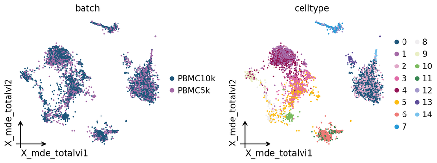
Corrected embedding#
Every backend writes its corrected representation to a stable obsm key — for this one it is adata.obsm['X_totalVI']. We project via ov.utils.mde for a lightweight UMAP-style display.
adata.obsm['X_mde_totalvi'] = ov.utils.mde(adata.obsm['X_totalVI'])
ov.pl.embedding(
    adata,
    basis='X_mde_totalvi',
    color=['batch', 'celltype'],
    frameon='small',
    wspace=0.5,
)
Key parameters#
Required:
protein_expression_obsm_key— name of the obsm slot with the protein matrix.
Architecture (→ scvi.model.TOTALVI.__init__):
n_latent,gene_dispersion,protein_dispersion,gene_likelihood,latent_distribution.
Optimisation (→ scvi.model.TOTALVI.train):
max_epochs,batch_size,early_stopping,accelerator.